Setup

In general, we will write a system of \(M\) simultaneous equations for \(M\) endogenous variables \(y_{1,t}\), …, \(y_{M,t}\) and \(K\) exogenous variables² \(x_{1,t}\), …, \(x_{K,t}\) in its structural form as:³ \[ \begin{aligned} \gamma_{11} y_{1,t} + \cdots + \gamma_{M1} y_{M,t} + \cdots + \beta_{11} x_{1,t} + \cdots + \beta_{K1} x_{K,t} =& \varepsilon_{1,t} \\ \gamma_{12} y_{1,t} + \cdots + \gamma_{M2} y_{M,t} + \cdots + \beta_{12} x_{1,t} + \cdots + \beta_{K2} x_{K,t} =& \varepsilon_{2,t} \\ \vdots& \\ \gamma_{1M} y_{1,t} + \cdots + \gamma_{MM} y_{M,t} + \cdots + \beta_{1M} x_{1,t} + \cdots + \beta_{KM} x_{K,t} =& \varepsilon_{M,t} \end{aligned} \] which we can write more succinctly as \[ \mathbf{y}_t' \boldsymbol{\Gamma} + \mathbf{x}_t' \mathbf{B} = \boldsymbol{\varepsilon}_t' \]

We can solve this system for the \(M\) endogenous variables \(\mathbf{y}\) by post-multiplying by \(\boldsymbol{\Gamma}^{-1}\): \[ \begin{aligned} \mathbf{y}_t' \boldsymbol{\Gamma} + \mathbf{x}_t' \mathbf{B} &= \boldsymbol{\varepsilon}_t' \\[0.4em] \mathbf{y}_t' \boldsymbol{\Gamma}\boldsymbol{\Gamma}^{-1} + \mathbf{x}_t' \mathbf{B}\boldsymbol{\Gamma}^{-1} &= \boldsymbol{\varepsilon}_t'\boldsymbol{\Gamma}^{-1} \\[0.4em] \mathbf{y}_t' &= - \mathbf{x}_t' \mathbf{B}\boldsymbol{\Gamma}^{-1} + \boldsymbol{\varepsilon}_t'\boldsymbol{\Gamma}^{-1} \\[0.4em] \mathbf{y}_t' &= \mathbf{x}_t' \boldsymbol{\Pi} + \mathbf{v}_t' \end{aligned} \] which gives our reduced-form equations.

Finally, to take into account our \(T\) observations, \[ \begin{bmatrix} \mathbf{Y} & \mathbf{X} & \mathbf{E} \end{bmatrix} = \begin{bmatrix} \mathbf{y}_1' & \mathbf{x}_1' & \boldsymbol{\varepsilon}_1' \\ \mathbf{y}_2' & \mathbf{x}_2' & \boldsymbol{\varepsilon}_2' \\ \vdots & \vdots & \vdots \\ \mathbf{y}_T' & \mathbf{x}_T' & \boldsymbol{\varepsilon}_T' \\ \end{bmatrix} \] which gives us \[ \mathbf{Y} \boldsymbol{\Gamma} + \mathbf{X} \mathbf{B} = \mathbf{E} \] We will assume strict exogeneity, \(\mathop{\boldsymbol{E}}\left[ \mathbf{E} | \mathbf{X} \right] = 0\). The reduced form is \[ \mathbf{Y} = \mathbf{X} \boldsymbol{\Pi} + \mathbf{V} \]

Identification: The problem

We can easily and consistently estimate the parameters from the reduced-form equations (\(\boldsymbol{\Pi}\)) via \(\hat{\boldsymbol{\Pi}} = (\mathbf{X}'\mathbf{X})^{-1} \mathbf{X}' \mathbf{Y}\). However, we usually want to learn about the structural parameters—not the reduced-form parameters. You might be tempted to think we can simply back out consistent estimates for the structural parameters using out consistent estimates for the reduced-form parameters. But there’s a problem here: our reduced-form equation does not guarantee a unique set of structural estimates. Observe:

1. Recall that \(\boldsymbol{\Pi} = - \mathbf{B} \boldsymbol{\Gamma}^{-1}\).
2. Post-multiply our structural equation by some arbitrary nonsingular matrix \(\mathbf{F}\): \[ \begin{aligned} \mathbf{Y} \boldsymbol{\Gamma} \mathbf{F} + \mathbf{X} \mathbf{B} \mathbf{F} &= \mathbf{E} \mathbf{F} \\ \mathbf{Y} \tilde{\boldsymbol{\Gamma}} + \mathbf{X} \tilde{\mathbf{B}} &= \tilde{\mathbf{E}} \end{aligned} \]
3. Solve for the reduced form of this alternate structural model: \[ \begin{aligned} \mathbf{Y} \tilde{\boldsymbol{\Gamma}} \tilde{\boldsymbol{\Gamma}}^{-1} + \mathbf{X} \tilde{\mathbf{B}} \tilde{\boldsymbol{\Gamma}}^{-1} &= \tilde{\mathbf{E}}\tilde{\boldsymbol{\Gamma}}^{-1} \\[0.2em] \mathbf{Y} &= - \mathbf{X} \mathbf{B} \mathbf{F} \mathbf{F}^{-1} \boldsymbol{\Gamma}^{-1} + \mathbf{E} \mathbf{F} \mathbf{F}^{-1} \boldsymbol{\Gamma}^{-1} \\[0.2em] \mathbf{Y} &= - \mathbf{X} \mathbf{B} \boldsymbol{\Gamma}^{-1} + \mathbf{E} \boldsymbol{\Gamma}^{-1} \\[0.2em] \mathbf{Y} &= \mathbf{X} \boldsymbol{\Pi} + \mathbf{V} \end{aligned} \]

Thus, the two different sets of structural equations produce the same reduced form. This result is bad news if you are trying to learn anything about the structural-form parameters. So what can we do? We need to make some assumptions/exclusions that allow us to rule out any \(\mathbf{F}\) except for the identity matrix.

Another way to think about this problem: We know that we can consistently estimate the \(K \times M\) reduced-form parameters and the \(M\times M\) reduced-form covariance matrix, which means we “know” \(KM + \frac{1}{2}(M+1)M\) parameters. We want to know the \(M\times M\) parameters in \(\boldsymbol{\Gamma}\), the \(K\times M\) parameters in \(\mathbf{B}\), and the \(M\times M\) parameters in \(\boldsymbol{\Sigma}\)—meaning we do not know \(M^2 + KM + \dfrac{1}{2}(M+1)M\) structural parameters. The difference between the numbers of “known” and “unknown” parameters is \(M^2\)—there are \(M^2\) more unknown parameters than known parameters. Hence the need to make some assumptions.

Identification: The solution(s)

Max and Greene provide a list of five solutions to our identification problem.

1. Normalization
2. Identities
3. Exclusions
4. Linear restrictions
5. Restriction on the disturbance covariance matrix

We’ll focus on (1) and (2–4).

Checking identification

Woolridge⁹ provides a nice four-step process for checking whether the \(i\)^th equation in the system is identified:

1. Set one of the parameters for the endogenous variables (i.e., one of the \(\gamma_{mi}\)) to one (normalization).
2. Define the \(J_i \times (M+K)\) matrix \(\mathbf{R}_i\) that imposes all of the restrictions for equation \(i\).
3. If \(J_i < M-1\), then equation \(i\) is not identified (under identified).
4. If \(J_i \geq M-1\), then equation \(i\) might be identified.
   • Let \(\boldsymbol{\Delta}\) be the matrix of all structural parameters with only the normalization restrictions applied.
   • Compute \(\mathbf{R}_i \boldsymbol{\Delta}\).
   • Impose the restrictions in the entire system.
   • Check the rank condition, i.e., \(\text{rank}\big(\mathbf{R}_i \boldsymbol{\Delta}\big) = M-1\).

Parameterization

We can use this reduced form to generate data, but first we need to define some parameters. \[ \begin{aligned} y_{1} &= 2 y_{2} + 3 x_2 + 5 x_3 + \varepsilon_1 \\ y_{2} &= 3 y_{3} + 1 x_1 + 4 x_2 + \varepsilon_2 \\ y_{3} &= 1 y_{1} + 2 x_1 + \varepsilon_3 \end{aligned} \]

Thus, the parameters in \(\boldsymbol{\Gamma}\) are: \[ \boldsymbol{\Gamma} = \begin{bmatrix} -1 & 0 & \gamma_{13} \\ \gamma_{21} & -1 & 0 \\ 0 & \gamma_{32} & -1 \end{bmatrix} = \begin{bmatrix} -1 & 0 & 1 \\ 2 & -1 & 0 \\ 0 & 3 & -1 \end{bmatrix} \] And the parameters in \(\mathbf{B}\) are: \[ \mathbf{B} = \begin{bmatrix} 0 & \beta_{12} & \beta_{13} \\ \beta_{21} & \beta_{22} & 0 \\ \beta_{31} & 0 & 0 \end{bmatrix} = \begin{bmatrix} 0 & 1 & 2 \\ 3 & 4 & 0 \\ 5 & 0 & 0 \end{bmatrix} \]

Now let’s set it all up in R.

First the general setup.

# General R setup ----
# Options
options(stringsAsFactors = F)
# Load new packages
library(pacman)
p_load(ggmap, leaflet)
# Load old packages
p_load(dplyr, ggplot2, ggthemes, parallel, magrittr, viridis)
# My ggplot2 theme
theme_ed <- theme(
  legend.position = "bottom",
  panel.background = element_rect(fill = NA),
  # panel.border = element_rect(fill = NA, color = "grey75"),
  axis.ticks = element_line(color = "grey95", size = 0.3),
  panel.grid.major = element_line(color = "grey95", size = 0.3),
  panel.grid.minor = element_line(color = "grey95", size = 0.3),
  legend.key = element_blank())
# My directories
dir_14 <- "/Users/edwardarubin/Dropbox/Teaching/ARE212/Section14/"

Now the structural parameters.

# Define the structural parameters ----
# Gamma
Gamma <- matrix(
  data = c(-1, 0, 1, 2, -1, 0, 0, 3, -1),
  nrow = 3,
  byrow = T
)
# Beta
Beta <- matrix(
  data = c(0, 1, 2, 3, 4, 0, 5, 0, 0),
  nrow = 3,
  byrow = T
)

Generate data

Now let’s generate the three \(x_k\) variables and the disturbances \(\varepsilon_{m}\) from standard random normal distributions. We want 10,000 observations.

# Generate data ----
# Set the sample size
N <- 1e3
# Set a seed
set.seed(12345)
# Generate the data for X and E
x_df <- data_frame(
  x1 = rnorm(N),
  x2 = rnorm(N),
  x3 = rnorm(N)
)
e_df <- data_frame(
  e1 = rnorm(N),
  e2 = rnorm(N),
  e3 = rnorm(N)
)

Now we will use the reduced form to generate our \([\mathbf{y}_1,\, \mathbf{y}_2,\, \mathbf{y}_3]\) variables.

# Generate the y variables
y_mat <- (-1) * as.matrix(x_df) %*% Beta %*% solve(Gamma) -
  as.matrix(e_df) %*% solve(Gamma)
# Force to data frame
y_df <- y_mat %>% as_data_frame()
names(y_df) <- c("y1", "y2", "y3")
# Join the data together
the_df <- bind_cols(y_df, x_df)

Estimation

Let’s estimate the parameters in the first equation. Keep in mind that truth in this simulation is \(\gamma_{21} = 2\), \(\beta_{21} = 3\), and \(\beta_{31} = 5\).

# The LHS variable in eq. 1
yi <- y_mat[,1]
# The RHS variables in eq. 1
Zi <- bind_cols(y_df[,2], x_df[,2:3]) %>% as.matrix()
# OLS estimates
solve(t(Zi) %*% Zi) %*% t(Zi) %*% yi

##        [,1]
## y2 1.802818
## x2 2.479916
## x3 4.388147

# Matrix of all exogenous variables in the system
X <- x_df %>% as.matrix()
# First-stage fitted values
Zi_hat <- X %*% solve(t(X) %*% X) %*% t(X) %*% Zi
# 2SLS estimates
solve(t(Zi_hat) %*% Zi_hat) %*% t(Zi_hat) %*% yi

##        [,1]
## y2 2.017908
## x2 3.049772
## x3 5.022968

Simulation

We’ve observed that in a single sample 2SLS gets us much closer to the true parameter estimates than OLS. Let’s use a simulation to confirm that this empirical observation (and the underlying theory) repeat through many samples.¹⁰

For this simulation, we want to

1. Generate a population of size \(N\)
2. Sample from the population with sample size \(n\)
3. Estimate OLS and 2SLS on the sample
4. Repeat 10,000 times

First, let’s generate the population. I think a 100,000 members will suffice. We can simply steal code from above.

# Simulation ----
# Clean up from the other 'simulation'
rm(N, x_df, e_df, y_mat, y_df, the_df, yi, Zi, X, Zi_hat); gc()

##           used (Mb) gc trigger (Mb) max used (Mb)
## Ncells  745519 39.9    1168576 62.5  1168576 62.5
## Vcells 1193138  9.2    2928070 22.4  2346069 17.9

# Generate population data:
# Set the population size
N <- 1e5
# Set a seed
set.seed(12345)
# Generate the data for X and E
pop_x <- data_frame(
  x1 = rnorm(N),
  x2 = rnorm(N),
  x3 = rnorm(N)
)
pop_e <- data_frame(
  e1 = rnorm(N),
  e2 = rnorm(N),
  e3 = rnorm(N)
)
# Generate the y variables
pop_y <- (-1) * as.matrix(pop_x) %*% Beta %*% solve(Gamma) -
  as.matrix(pop_e) %*% solve(Gamma)
# Force to data frame
y_df <- pop_y %>% as_data_frame()
names(y_df) <- c("y1", "y2", "y3")
# Join the data together
pop_df <- bind_cols(y_df, pop_x)
# Clean up
rm(pop_x, pop_e, pop_y, y_df); gc()

##           used (Mb) gc trigger (Mb) max used (Mb)
## Ncells  745647 39.9    1168576 62.5  1168576 62.5
## Vcells 1793263 13.7    2928070 22.4  2904307 22.2

Now we will write a function that carries out tasks (2) and (3).

# Function: Run a single iteration of the simulation
fun_iter <- function(i, data, sample_size) {
  # Sample from the population
  smpl_df <- sample_n(tbl = data, size = sample_size)
  # The LHS variable in eq.1
  yi <- smpl_df %>% select(y1) %>% as.matrix()
  # The RHS variables in eq. 1
  Zi <- smpl_df %>% select(y2, x2, x3) %>% as.matrix()
  # OLS estimates
  d_ols <- solve(t(Zi) %*% Zi) %*% t(Zi) %*% yi
  # Matrix of all exogenous variables in the system
  X <- smpl_df %>% select(starts_with("x")) %>% as.matrix()
  # First-stage fitted values
  Zi_hat <- X %*% solve(t(X) %*% X) %*% t(X) %*% Zi
  # 2SLS estimates
  d_2sls <- solve(t(Zi_hat) %*% Zi_hat) %*% t(Zi_hat) %*% yi
  # Create results data frame
  result_df <- rbind(t(d_ols), t(d_2sls)) %>% as_data_frame()
  # Add method and iteration variables
  result_df %<>% mutate(
    method = c("OLS", "2SLS"),
    iter = i
  )
  # Return the results
  return(result_df)
}

Now for the simulation! We will run 10,000 iterations with sample size 1,000. It takes about a minute to run on my machine using three cores (I’m using proc.time() to track the start and end times of the simulation. Taking the difference gives us the elapsed time during the simulation.).

t1 <- proc.time()
# Run fun_iter() 10,000 times
sim_df <- mclapply(
  X = 1:1e4,
  FUN = fun_iter,
  mc.cores = 3,
  data = pop_df,
  sample_size = 1e3
) %>% bind_rows()
t2 <- proc.time()
t2 - t1

##    user  system elapsed 
##  97.428  17.244  59.905

Finally, let’s plot our results. First, \(\gamma_{21}\)—the coefficient on \(y_2\) in the first equation—which we know is actually equal to 2.

ggplot(data = sim_df, aes(x = y2, fill = method)) +
  geom_density(color = NA, alpha = 0.9) +
  geom_vline(xintercept = Gamma[2,1], color = viridis(3, option = "C")[2]) +
  geom_hline(yintercept = 0, color = "black") +
  labs(
    x = expression(Parameter~estimates:~gamma[21]),
    y = "Density"
  ) +
  ggtitle(
    expression(paste("Simultaneity bias: Comparing OLS and 2SLS in estimating equation 1 parameter ",
      gamma[21])),
    subtitle = "10,000 iterations with sample size 1,000"
  ) +
  scale_fill_viridis(
    "Estimation method:",
    discrete = T, option = "C", begin = 0.15, end = 0.85
  ) +
  theme_ed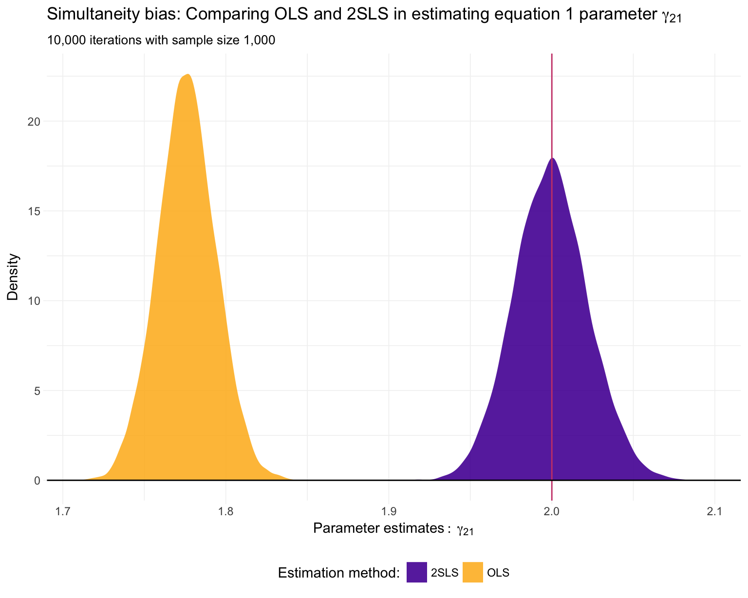

Repeat for \(\beta_{21}\) (\(=3\)) and \(\beta_{31}\) (\(=5\)).

ggplot(data = sim_df, aes(x = x2, fill = method)) +
  geom_density(color = NA, alpha = 0.9) +
  geom_vline(xintercept = Beta[2,1], color = viridis(3, option = "C")[2]) +
  geom_hline(yintercept = 0, color = "black") +
  labs(
    x = expression(Parameter~estimates:~beta[21]),
    y = "Density"
  ) +
  ggtitle(
    expression(paste("Simultaneity bias: Comparing OLS and 2SLS in estimating equation 1 parameter ",
      beta[21])),
    subtitle = "10,000 iterations with sample size 1,000"
  ) +
  scale_fill_viridis(
    "Estimation method:",
    discrete = T, option = "C", begin = 0.15, end = 0.85
  ) +
  theme_ed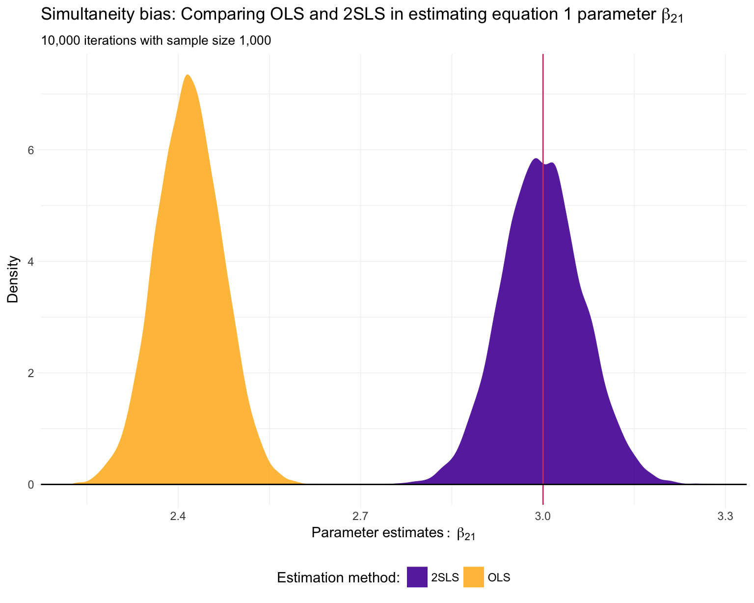

ggplot(data = sim_df, aes(x = x3, fill = method)) +
  geom_density(color = NA, alpha = 0.9) +
  geom_vline(xintercept = Beta[3,1], color = viridis(3, option = "C")[2]) +
  geom_hline(yintercept = 0, color = "black") +
  labs(
    x = expression(Parameter~estimates:~beta[31]),
    y = "Density"
  ) +
  ggtitle(
    expression(paste("Simultaneity bias: Comparing OLS and 2SLS in estimating equation 1 parameter ",
      beta[31])),
    subtitle = "10,000 iterations with sample size 1,000"
  ) +
  scale_fill_viridis(
    "Estimation method:",
    discrete = T, option = "C", begin = 0.15, end = 0.85
  ) +
  theme_ed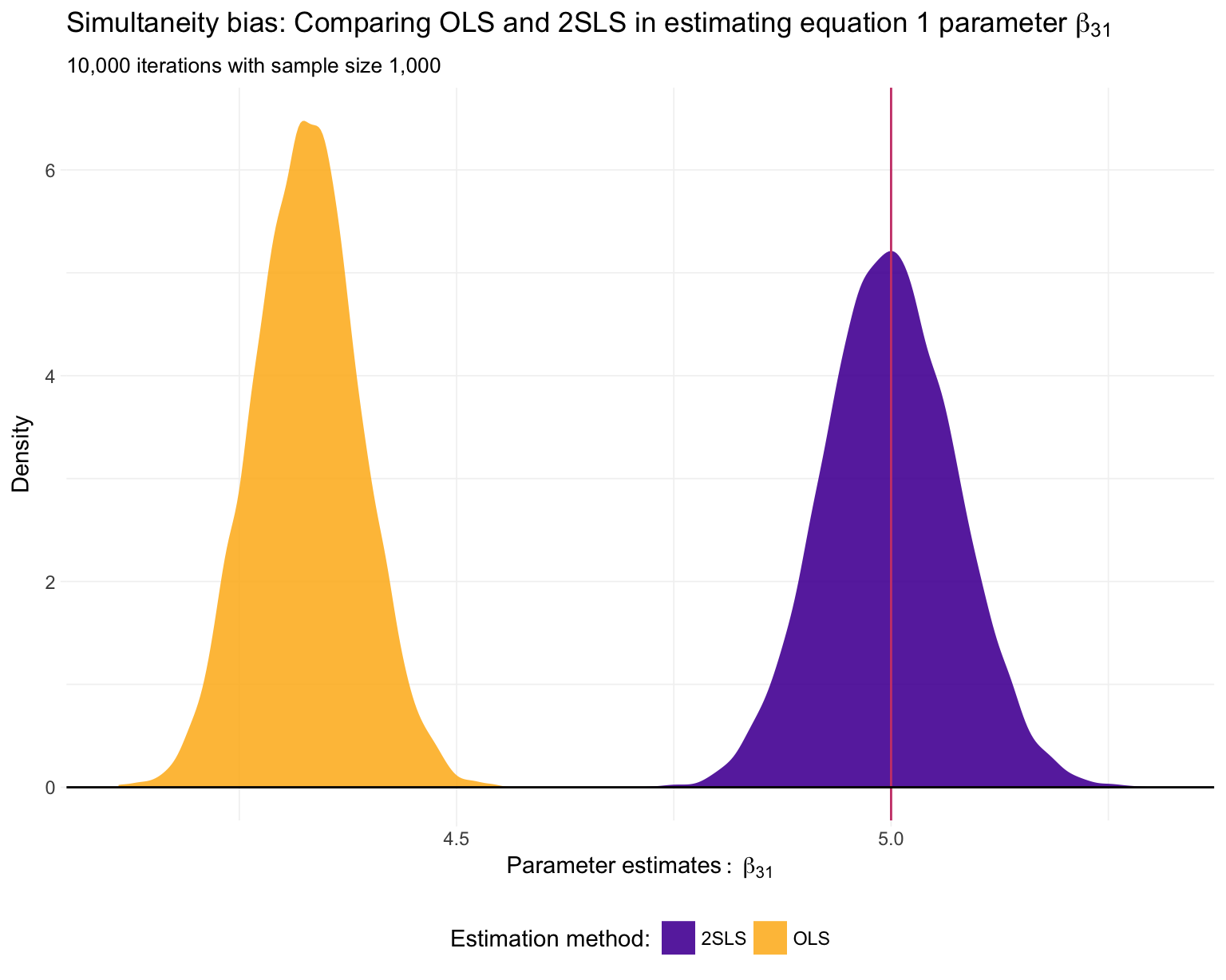

Just as we suspected: 2SLS is providing consistent¹¹ estimates of the structural parameters, while OLS is inconsistent in each application.