Follow ups

library(pacman)
p_load(dplyr)
x <- data.frame(a = c(1:4, NA), b = c("..", 1, 2, 3, ".."))  %>% as_tibble()
x

## # A tibble: 5 x 2
##       a b    
##   <int> <fct>
## 1     1 ..   
## 2     2 1    
## 3     3 2    
## 4     4 3    
## 5    NA ..

x <- data.frame(a = c(1:4, NA), b = c("..", 1, 2, 3, ".."))  %>% as_tibble()
x[x == ".."] <- NA
x

## # A tibble: 5 x 2
##       a b    
##   <int> <fct>
## 1     1 <NA> 
## 2     2 1    
## 3     3 2    
## 4     4 3    
## 5    NA <NA>

# Define our function
rep_na <- function(y) replace(y, which(y == ".."), NA)

# Make some data
x <- data.frame(a = c(1:4, NA), b = c("..", 1, 2, 3, ".."))  %>% as_tibble()
# Replace .. with NA
x %>% mutate(b = rep_na(b) %>% as.numeric())

## # A tibble: 5 x 2
##       a     b
##   <int> <dbl>
## 1     1   NA 
## 2     2    2.
## 3     3    3.
## 4     4    4.
## 5    NA   NA

# Make some data
x <- data.frame(a = c(1:4, NA), b = c("..", 1, 2, 3, ".."))  %>% as_tibble()
# Replace .. with NA
x %>% mutate_all(rep_na) %>% mutate_all(as.numeric)

## # A tibble: 5 x 2
##       a     b
##   <dbl> <dbl>
## 1    1.   NA 
## 2    2.    2.
## 3    3.    3.
## 4    4.    4.
## 5   NA    NA

What you will need

Packages:

• Previously used: dplyr, lfe, readr
• New: magrittr and parallel (parallel is likely already installed)

Data: The auto.csv file.

Review: It will also be helpful if you review the simulations from section 3 and section 4.

Last week

In our previous section, we discussed logical operators, optional arguments to functions, the Frisch-Waugh-Lovell theorem (and its applications—omitted variable bias, bad controls), and R²/measures of fit.

This week

Testing hypotheses in R! Plus simulation and parallelizing your code.

Setting up

As we discussed before, I find it helpful to have a section of my R script where I set settings, load libraries, define directories, read data.

# Settings
options(stringsAsFactors = F)
# Packages
library(pacman)
p_load(dplyr, lfe, magrittr, readr)
# Directories
dir_data <- "/Users/edwardarubin/Dropbox/Teaching/ARE212/Section05/"
# Load the dataset from CSV
cars <- paste0(dir_data, "auto.csv") %>% read_csv()

We should also load the functions that we will want to use:

# Functions ----
# Function to convert tibble, data.frame, or tbl_df to matrix
to_matrix <- function(the_df, vars) {
  # Create a matrix from variables in var
  new_mat <- the_df %>%
    # Select the columns given in 'vars'
    select_(.dots = vars) %>%
    # Convert to matrix
    as.matrix()
  # Return 'new_mat'
  return(new_mat)
}
# Function for OLS coefficient estimates
b_ols <- function(data, y_var, X_vars, intercept = TRUE) {
  # Require the 'dplyr' package
  require(dplyr)
  # Create the y matrix
  y <- to_matrix(the_df = data, vars = y_var)
  # Create the X matrix
  X <- to_matrix(the_df = data, vars = X_vars)
  # If 'intercept' is TRUE, then add a column of ones
  if (intercept == T) {
    # Bind a column of ones to X
    X <- cbind(1, X)
    # Name the new column "intercept"
    colnames(X) <- c("intercept", X_vars)
  }
  # Calculate beta hat
  beta_hat <- solve(t(X) %*% X) %*% t(X) %*% y
  # Return beta_hat
  return(beta_hat)
}

magrittr

Notice that we loaded a new package called magrittr. We’ll talk about its functions shortly. magrittr offers is more flexibility for piping commands—similar to dplyr’s pipe %>%. Fun facts: the package’s name comes from the Belgian artist René Magritte. Specifically, the package is referencing Magritte’s painting “The Treachery of Images,” which shows a pipe and the caption “This is not a pipe.” Get it?

\(t\) tests

Before we get to the math, you should know that a Guinness brewer named William S. Gosset developed the t test to deal with the fact that his sample means did not act normally. More.

Okay. Now let’s math it up.

Suppose we want to test whether the j^th coefficient \(\beta_j\) in our model is is significantly different from some other value \(\bar\gamma\), using the significance level \(\alpha\). Following Max’s notes, we can calculate the t statistic for the j^th coefficient as

\[ t_j = \dfrac{b_j - \bar\gamma}{\sqrt{ s^2 \cdot \left\{ \left(\mathbf{X}^\prime\mathbf{X}\right)^{-1} \right\}_{jj} }} = \dfrac{b_j - \bar\gamma}{\text{se}\left(b_j\right)} \]

where \(b_j\) is our estimate for \(\beta_j\), \(s^2\) is our estimate of \(\sigma^2\), and \(\left\{ \left(\mathbf{X}^\prime\mathbf{X}\right)^{-1} \right\}_{jj}\) is the j^th diagonal element of \(\left(\mathbf{X}^\prime\mathbf{X}\right)^{-1}\).

Now let’s write a function in R that will calculate this test statistic.

t_stat <- function(data, y_var, X_vars, gamma, intercept = T) {
  # Turn data into matrices
  y <- to_matrix(data, y_var)
  X <- to_matrix(data, X_vars)
  # Add intercept if requested
  if (intercept == T) X <- cbind(1, X)
  # Calculate n and k for degrees of freedom
  n <- nrow(X)
  k <- ncol(X)
  # Estimate coefficients
  b <- b_ols(data, y_var, X_vars, intercept)
  # Calculate OLS residuals
  e <- y - X %*% b
  # Calculate s^2
  s2 <- (t(e) %*% e) / (n-k)
  # Force s2 to numeric
  s2 %<>% as.numeric()
  # Inverse of X'X
  XX_inv <- solve(t(X) %*% X)
  # Standard error
  se <- sqrt(s2 * diag(XX_inv))
  # Vector of _t_ statistics
  t_stats <- (b - gamma) / se
  # Return the _t_ statistics
  return(t_stats)
}

You could probably write the same function in a single (long) line of code. However, it would be (1) ugly and (2) difficult to debug. I recommend some intermediate steps—even if you are using pipes.

Now let’s test drive our function t_stat() on our car data.³ Specifically, let’s regress price on an intercept, weight, and mpg and test the estimated coefficients against the null hypothesis that they are zero, i.e., \(\bar{\boldsymbol{\gamma}} = \left[0 \quad 0 \quad 0\right]^\prime\).

We should probably compare our calculated t statistics to the t statistics calculated by the function felm(). For this task, we will grab the coefficients from the summary() function⁴ after it is applied to felm(). To grab the coefficients from summary() we will use the %$% operator from magrittr.

cor(cars$price, cars$weight)
## [1] 0.5386115
cars %$% cor(price, weight)
## [1] 0.5386115

t_stat(cars,
  y_var = "price", X_vars = c("mpg", "weight"),
  gamma = 0, intercept = T)

##                price
## intercept  0.5410180
## mpg       -0.5746808
## weight     2.7232382

felm(price ~ mpg + weight, cars) %>%
  summary() %$% (coefficients)[,3]

## (Intercept)         mpg      weight 
##   0.5410180  -0.5746808   2.7232382

p-values

What do we need to do to turn our newly calculated t statistics into p-values? First off, we are going to stick with two-sided hypothesis tests where the null hypothesis is our parameter is zero.⁶ We need to find the percentage of the t distribution (with \(n-k\) degrees of freedom) that is more extreme than (the absolute value) of our test statistic. More formally, the p-value \(p\) for our j^th t statistic \(t_j\) is defined as

\[ p = \text{Pr}\left( t_\text{df} > \left| t_j \right| \right) \times 2\]

Let’s code up the calculation of a p-value. We will make use of the function pt(q, df), which gives the distribution function for a t-distributed random variable evaluated at q with df degrees of freedom. In our situation, we will make use of pt()’s optional argument lower.tail. The lower.tail argument defaults to TRUE, which means pt() is evaluating the CDF at q. If we set the lower.tail argument to FALSE, then we will get one minus the CDF, which is what we want for the p-value.

Example

# The default: lower.tail = TRUE
pt(q = 2, df = 15)
## [1] 0.9680275
# Setting lower.tail = TRUE
pt(q = 2, df = 15, lower.tail = T)
## [1] 0.9680275
# Setting lower.tail = FALSE
pt(q = 2, df = 15, lower.tail = F)
## [1] 0.0319725

This situation is a great example of how R plays very nicely with vectors. Imagine we have a vector of t statistics named t_stats. We can calculate the p-values associated with the t statistics via

pt(q = abs(t_stats), df = n-k, lower.tail = F) * 2

Put it all together

Finally, let’s put together a nice-ish table like the one that felm() returns: coefficient estimates, standard errors, t statistics, and p-values. Because I’m so clever, we’ll call the function that performs this task ols().⁷ In addition, because many of our functions return matrices, we will use as.vector() to convert \(1\times k\) or \(k\times 1\) matrices to vectors. We will also use the round() function to maintain a reasonable number of digits.

ols <- function(data, y_var, X_vars, intercept = T) {
  # Turn data into matrices
  y <- to_matrix(data, y_var)
  X <- to_matrix(data, X_vars)
  # Add intercept if requested
  if (intercept == T) X <- cbind(1, X)
  # Calculate n and k for degrees of freedom
  n <- nrow(X)
  k <- ncol(X)
  # Estimate coefficients
  b <- b_ols(data, y_var, X_vars, intercept)
  # Calculate OLS residuals
  e <- y - X %*% b
  # Calculate s^2
  s2 <- (t(e) %*% e) / (n-k)
  # Update s2 to numeric
  s2 %<>% as.numeric()
  # Inverse of X'X
  XX_inv <- solve(t(X) %*% X)
  # Standard error
  se <- sqrt(s2 * diag(XX_inv))
  # Vector of _t_ statistics
  t_stats <- (b - 0) / se
  # Calculate the p-values
  p_values = pt(q = abs(t_stats), df = n-k, lower.tail = F) * 2
  # Nice table (data.frame) of results
  results <- data.frame(
    # The rows have the coef. names
    effect = rownames(b),
    # Estimated coefficients
    coef = as.vector(b) %>% round(3),
    # Standard errors
    std_error = as.vector(se) %>% round(3),
    # t statistics
    t_stat = as.vector(t_stats) %>% round(3),
    # p-values
    p_value = as.vector(p_values) %>% round(4)
    )
  # Return the results
  return(results)
}

Finally, let’s test our function and compare it to the output of felm() and the coefficients it outputs in summary().

ols(data = cars,
  y_var = "price",
  X_vars = c("mpg", "weight"),
  intercept = T)
##      effect     coef std_error t_stat p_value
## 1 intercept 1946.069  3597.050  0.541  0.5902
## 2       mpg  -49.512    86.156 -0.575  0.5673
## 3    weight    1.747     0.641  2.723  0.0081

felm(price ~ mpg + weight, cars) %>%
  summary() %$% coefficients
##                Estimate   Std. Error    t value    Pr(>|t|)
## (Intercept) 1946.068668 3597.0495988  0.5410180 0.590188628
## mpg          -49.512221   86.1560389 -0.5746808 0.567323727
## weight         1.746559    0.6413538  2.7232382 0.008129813

Pretty cool, eh?

The formal part

Assume our data-generating process is

\[ \mathbf{y} = \beta_0 + \mathbf{x}_1 \beta_1 + \mathbf{x}_2 \beta_2 + \mathbf{x}_3 \beta_3 + \varepsilon \]

To test whether \(\beta_1\), \(\beta_2\), and \(\beta_3\) are jointly different from zero, we need two more objects: \(\mathbf{R}\) and \(\mathbf{r}\). \(\mathbf{R}\) is a \(j\times k\) matrix where \(j\) is the number of joint hypotheses we will test and \(k\) is the number of coefficients in our model (inclusive of the intercept). The \(\mathbf{R}\) matrix creates linear combinations of the coefficients for each of individual hypotheses that we will jointly test. The \(j\times 1\) vector \(\mathbf{r}\) gives the right-hand side of the hypotheses that we want to test.

For example, if we want to jointly test \(\beta_1 = 1\), \(\beta_2 = 0\) and \(\beta_3 = 7\), our matrices would be⁹

\[ \mathbf{R} = \left[ \begin{array}{cccc} 0 & 1 & 0 & 0 \\ 0 & 0 & 1 & 0 \\ 0 & 0 & 0 & 1 \\ \end{array} \right] \enspace \text{and} \enspace \mathbf{r} = \left[ \begin{array}{c} 1 \\ 0 \\ 7 \\ \end{array} \right] \]

If we want to jointly test that \(\beta_1\), \(\beta_2\), and \(\beta_3\) are jointly different from zero, the matrices become

\[ \mathbf{R} = \left[ \begin{array}{cccc} 0 & 1 & 0 & 0 \\ 0 & 0 & 1 & 0 \\ 0 & 0 & 0 & 1 \\ \end{array} \right] \enspace \text{and} \enspace \mathbf{r} = \left[ \begin{array}{c} 0 \\ 0 \\ 0 \\ \end{array} \right] \]

As you saw in lecture, you can write the statistic in the \(F\) test as

\[ F = \dfrac{(\mathbf{R}\mathbf{b}-\mathbf{r})^\prime \left[\mathbf{R}\left(\mathbf{X}^\prime \mathbf{X}\right)^{-1} \right] (\mathbf{R}\mathbf{b}-\mathbf{r}) / J}{s^2} = \dfrac{(\mathbf{R}\mathbf{b})^\prime \left[\mathbf{R}\left(\mathbf{X}^\prime \mathbf{X}\right)^{-1} \right] (\mathbf{R}\mathbf{b}) / J}{s^2} \]

where the equality comes from the special (though common) case of \(\mathbf{r} = \boldsymbol{0}\). In our case, \(J=3\) because we are jointly testing three hypotheses (also called imposing three restrictions).

\(F\) in R

Now we will write up a function that jointly tests all of the coefficients (except the intercept). Here, I will assume the joint hypotheses in which we are interested take the from \(\beta_i = 0\). You should feel free to write more complex functions that take an arbitrary \(\mathbf{R}\) and \(\mathbf{r}\). I’m also going to assume that we want an intercept.

joint_test <- function(data, y_var, X_vars) {
  # Turn data into matrices
  y <- to_matrix(data, y_var)
  X <- to_matrix(data, X_vars)
  # Add intercept
  X <- cbind(1, X)
  # Name the new column "intercept"
  colnames(X) <- c("intercept", X_vars)
  # Calculate n and k for degrees of freedom
  n <- nrow(X)
  k <- ncol(X)
  # J is k-1
  J <- k - 1
  # Create the R matrix: bind a column of zeros
  # onto a J-by-J identity matrix
  R <- cbind(0, diag(J))

  # Estimate coefficients
  b <- b_ols(data, y_var, X_vars)
  # Calculate OLS residuals
  e <- y - X %*% b
  # Calculate s^2
  s2 <- (t(e) %*% e) / (n-k)
  # Force s2 to numeric
  s2 %<>% as.numeric()

  # Create the inner matrix R(X'X)^(-1)R'
  RXXR <- R %*% solve(t(X) %*% X) %*% t(R)
  # Calculate the F stat
  f_stat <- t(R %*% b) %*% solve(RXXR) %*% (R %*% b) / J / s2
  # Calculate the p-value
  p_value <- pf(q = f_stat, df1 = J, df2 = n-k, lower.tail = F)
  # Create a data.frame of the f stat. and p-value
  results <- data.frame(
    f_stat = f_stat %>% as.vector(),
    p_value = p_value %>% as.vector())
  return(results)
}

Now run the \(F\) test jointly testing the significance of the coefficients on miles per gallon and weight (with the outcome variable price).

joint_test(data = cars,
  y_var = "price", X_vars = c("mpg", "weight"))

##     f_stat      p_value
## 1 14.73982 4.424878e-06

Finally, let’s check if the our function matches felm()’s joint statistic and p-value.

felm(price ~ mpg + weight, cars) %>%
  summary() %$% F.fstat

##            F          df1          df2            p 
## 1.473982e+01 2.000000e+00 7.100000e+01 4.424878e-06

Warnings/messages

What if you want to incorporate this \(F\) statistic and joint test p-value in your ols() function? You might face a few challenges.

1. We created a nice table at the end of the ols() function. Where would we put this new output from the \(F\) test? One option is to use a list: you could return a list where the first element is our nice results table and the second element is the information from our \(F\) test.
2. The second challenge that you face is that our ols() function allows the user to select whether or not to include an intercept, but we need an intercept for our \(F\) test. Solution: warning and error messages in R.

For an extreme solution, you could write an if statement that checked whether the user specified intercept = F. If intercept is indeed FALSE, you could stop the function in its tracks and print the error message “No intercept!”. In code, this would look like

if (intercept == F) stop("No intercept!")

However, this solution is a bit extreme: you will not be able to get your results for the other parts of your function if intercept = F. Instead, you might want to use the warning() function to warn the user that because she/he requested no intercept, you will not return an \(F\) statistic or joint p-value. Let’s do it.

Below is a function ols_joint() that returns a list of results and issues a warning if the user specifies no intercept.

ols_joint <- function(data, y_var, X_vars, intercept = T) {
  # Run the ols() function
  ols_results <- ols(data, y_var, X_vars, intercept)
  # If intercept is T, run the joint_test() function
  # Otherwise, define joint_results to be NA and
  # issue a warning
  if (intercept == T) {
    joint_results <- joint_test(data, y_var, X_vars)
  } else {
    warning("No intercept: will not perform F test.")
    joint_results <- data.frame(
      f_stat = NA,
      p_value = NA)
  }
  # Create the results list
  results <- list(ols_results, joint_results)
  # Return the results list
  return(results)
}

Now let’s see what happens when we include and exclude an intercept.

With an intercept:

ols_joint(data = cars,
  y_var = "price",
  X_vars = c("mpg", "weight"),
  intercept = T)

## [[1]]
##      effect     coef std_error t_stat p_value
## 1 intercept 1946.069  3597.050  0.541  0.5902
## 2       mpg  -49.512    86.156 -0.575  0.5673
## 3    weight    1.747     0.641  2.723  0.0081
## 
## [[2]]
##     f_stat      p_value
## 1 14.73982 4.424878e-06

Without an intercept:

ols_joint(data = cars,
  y_var = "price",
  X_vars = c("mpg", "weight"),
  intercept = F)

## Warning in ols_joint(data = cars, y_var = "price", X_vars = c("mpg",
## "weight"), : No intercept: will not perform F test.

## [[1]]
##   effect   coef std_error t_stat p_value
## 1    mpg -5.479    28.122 -0.195  0.8461
## 2 weight  2.076     0.199 10.431  0.0000
## 
## [[2]]
##   f_stat p_value
## 1     NA      NA

Functions

The first function will generate data for the regression, given a sample size sample_size. As I mentioned above, we will stick with a simple linear regression

\[\mathbf{y} = \beta_0 + \beta_1 \mathbf{x} + \boldsymbol{\varepsilon}\]

Let’s assume \(\beta_0 = 7\) and \(\beta_1 = 0.5\). We will draw \(x\) and \(\varepsilon\) from the standard normal distribution.¹⁰

# Function to generate data
gen_data <- function(sample_size) {
  # Create data.frame with random x and error
  data_df <- data.frame(
    x = rnorm(sample_size),
    e = rnorm(sample_size))
  # Calculate y = 7 + 0.5 x + e; drop 'e'
  data_df %<>% mutate(y = 7 + 0.5 * x + e) %>%
    select(-e)
  # Return data_df
  return(data_df)
}

Now we will write a function that takes the output of gen_data() and feeds it to ols(), which gives us the coefficient estimates and p-value from testing the coefficients against zero.

one_sim <- function(sample_size) {
  # Estimate via OLS
  ols_est <- ols(data = gen_data(sample_size),
    y_var = "y", X_vars = "x")
  # Grab the estimated coefficient on x
  # (the second element of 'coef')
  b1 <- ols_est %$% coef[2]
  # Grab the second p-value
  # (the first p-value is for the intercept)
  p_value <- ols_est %$% p_value[2]
  # Return a data.frame with b1 and p_value
  return(data.frame(b1, p_value))
}

Finally, we need to write a function that will run the simulation n_sims times. One option we used previously is the lapply() function. I’ll provide you with an alternative here that uses replicate().¹¹ replicate() needs two arguments: the number of replications (n) and the expression (expr) you would like to replicate. You can also give replicate() an argument called simplify which tells the function how to format the results (which type of class). I prefer setting simplify = F so that I know I will get a list. We can then use bind_rows() on the list to create a nice data frame.

The function will require two arguments: n_sims, the number of simulations that we want to run, and n, the sample size drawn within each simulation. The function will also accept a third optional argument seed, which is the seed we will use in the simulation. The default value for seed will be 12345.

ols_sim <- function(n_sims, sample_size, seed = 12345) {
  # Set the seed
  set.seed(seed)
  # Run one_sim n_sims times; convert results to data.frame
  sim_df <- replicate(
    n = n_sims,
    expr = one_sim(sample_size),
    simplify = F
    ) %>% bind_rows()
  # Return sim_df
  return(sim_df)
}

Finally, let’s run the ols_sim() function for two different sample sizes: 10 and 100. For each sample size, we will run the simulation 1,000 times.

Warning: Running two-thousand iterations of a simulation can take some time.

# Run ols_sim for sample size of 10
sim10 <- ols_sim(n_sims = 1e3, sample_size = 10)
# Run ols_sim for sample size of 100
sim100 <- ols_sim(n_sims = 1e3, sample_size = 100)

Graphs

Let’s look at our results. I’m going to use the ggplot2 package. Don’t worry about the coding syntax for the moment: we will cover ggplot2 next section. For now, just look at the (pretty) pictures.¹²

p_load(ggplot2, ggthemes)

Density plot of the p-values for the sample-size 10 simulation

ggplot(data = sim10, aes(x = p_value)) +
  stat_density(fill = "grey20", alpha = 0.9) +
  geom_vline(xintercept = 0.05, color = "deeppink2", size = 1) +
  theme_pander() +
  xlab(expression(paste(italic("p"), "-Value"))) +
  ylab("Density") +
  ggtitle(expression(paste("Distribution of ", italic(p),
    "-Values from 1,000 simulations with sample size 10")))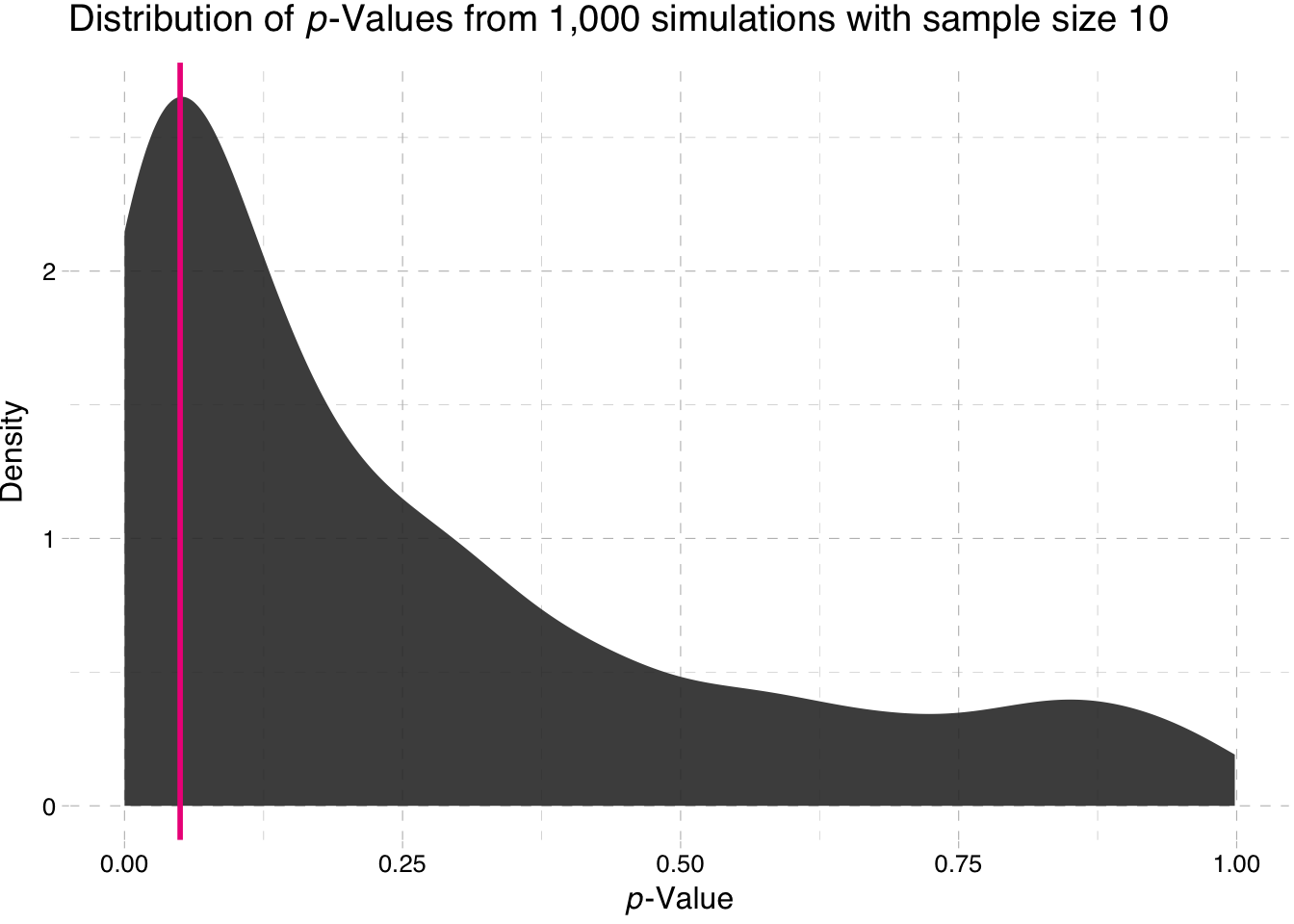

Density plot of the p-values for the sample-size 100 simulation

ggplot(data = sim100, aes(x = p_value)) +
  stat_density(fill = "grey20", alpha = 0.9) +
  geom_vline(xintercept = 0.05, color = "deeppink2", size = 1) +
  xlim(0, 0.1) +
  theme_pander() +
  xlab(expression(paste(italic("p"), "-Value"))) +
  ylab("Density") +
  ggtitle(expression(paste("Distribution of ", italic(p),
    "-Values from 1,000 simulations with sample size 100")))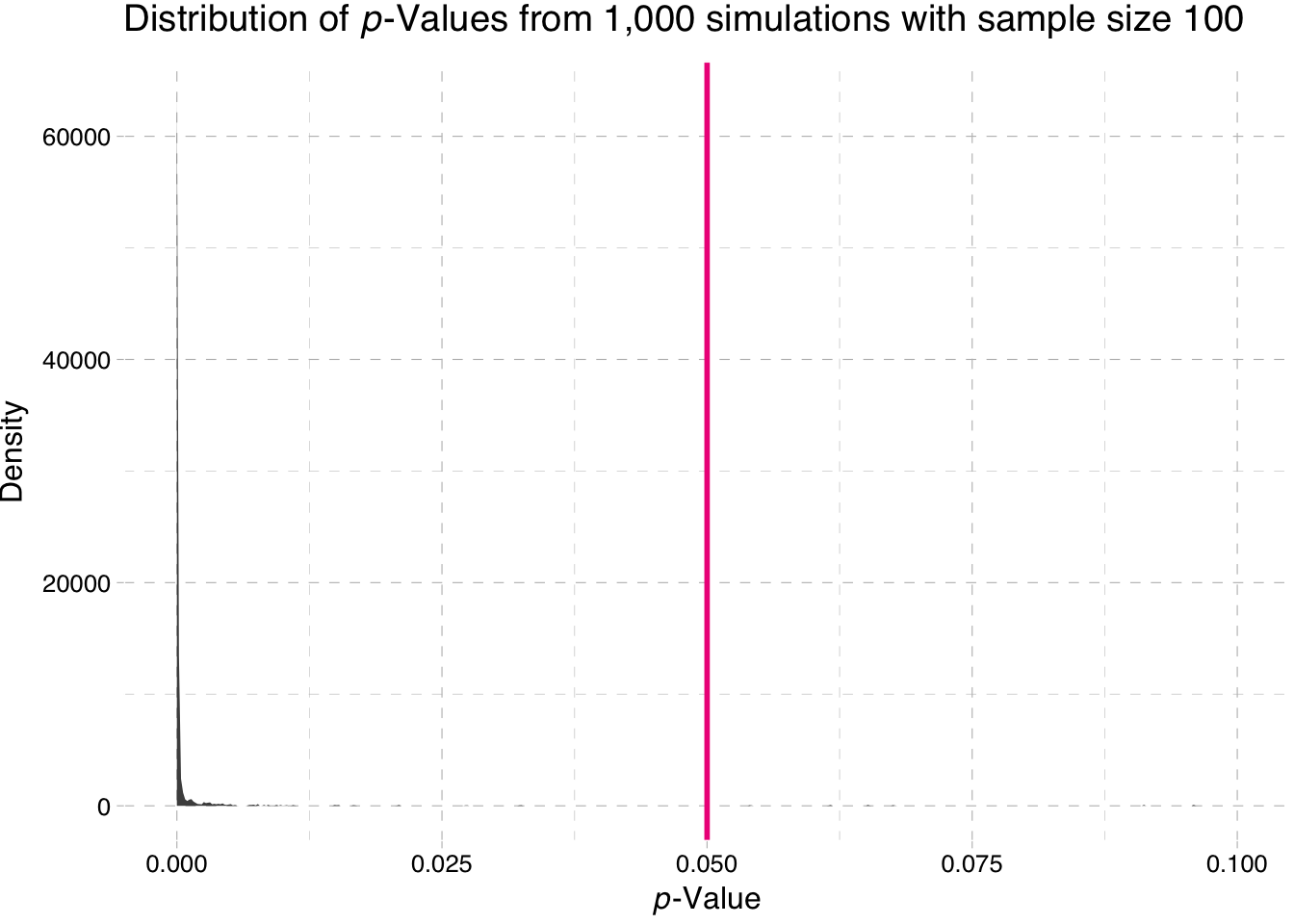

So what is the takeaway here? Power increases with sample size. Why does the second plot look so strange? Nearly all of the p-values are approximately zero.

A related topic: How does sample size affect the distribution of estimates for \(\beta_1\)?

Density plot of the estimates for \(\beta_1\) for sample-size 10 simulation

ggplot(data = sim10, aes(x = b1)) +
  stat_density(fill = "grey70") +
  geom_vline(xintercept = 0.5, color = "darkviolet", size = 1) +
  theme_pander() +
  xlab(expression(paste(beta[1], " estimate"))) +
  ylab("Density") +
  ggtitle(expression(paste("Distribution of ", beta[1],
    " estimates from 1,000 simulations with sample size 10")))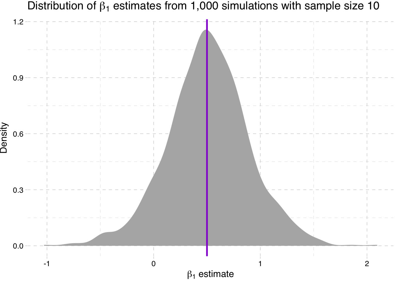

Density plot of the estimates for \(\beta_1\) for sample-size 100 simulation

ggplot(data = sim100, aes(x = b1)) +
  stat_density(fill = "grey70") +
  geom_vline(xintercept = 0.5, color = "darkviolet", size = 1) +
  theme_pander() +
  xlab(expression(paste(beta[1], " estimate"))) +
  ylab("Density") +
  ggtitle(expression(paste("Distribution of ", beta[1],
    " estimates from 1,000 simulations with sample size 100")))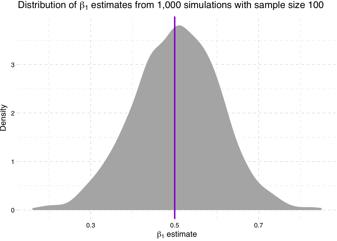

So what is going on here? We are seeing the distribution of the estimates for \(\beta_1\) get tighter around the true parameter value as the sample size increases (make sure you note the differences on the x-axis).

On Mac and Linux

You will need to install the parallel package. The parallel package offers a number of functions to parallelize your code, but today we will focus on the parallelized version of lapply(): mclapply(). After loading the parallel package, enter ?mclapply into the R console to see the function description. As you can see, mclapply() starts with the same two arguments as lapply()—X and FUN—and then offers a number of other options. The most important option for us at the moment is mc.cores, which is the option that allows you to choose how many processes to run simultaneously.

p_load(parallel)

While infinity would be a nice number to enter in the mc.cores argument, you should probably stick with a number less than or equal to the number of cores on your computer. To see how many cores are available on your machine, type detectCores() into the R console.

detectCores()

## [1] 4

Looks like I have four.¹³

We are now going to parallelize our function ols_sim(). For this parallelization, we will replace the replicate() function with a similar use of lapply(). However, instead of using plain old lapply(), we will use mclapply() with four cores.

ols_sim_mc <- function(n_sims, sample_size, seed = 12345) {
  # Require the parallel package
  require(parallel)
  # Set the seed
  set.seed(seed)
  # Run one_sim n_sims times; convert results to data.frame
  sim_df <- mclapply(
    X = rep(x = sample_size, times = n_sims),
    FUN = one_sim,
    # Specify that we want 4 cores
    mc.cores = 4
    ) %>% bind_rows()
  # Return sim_df
  return(sim_df)
}

Now let’s run the simulation again—both parallelized and non-parallelized. This time around, let’s go for 10,000 iterations. And let’s time everything (using proc.time() to get the time at which the simulation starts and stops).

Not parallelized:

# Run ols_sim for sample size of 10
start1 <- proc.time()
sim10 <- ols_sim(n_sims = 1e4, sample_size = 10)
stop1 <- proc.time()
# Run ols_sim for sample size of 100
start2 <- proc.time()
sim100 <- ols_sim(n_sims = 1e4, sample_size = 100)
stop2 <- proc.time()

Parallelized:

# Run ols_sim_mc for sample size of 10
start3 <- proc.time()
sim10_mc <- ols_sim_mc(n_sims = 1e4, sample_size = 10)
stop3 <- proc.time()
# Run ols_sim_mc for sample size of 100
start4 <- proc.time()
sim100_mc <- ols_sim_mc(n_sims = 1e4, sample_size = 100)
stop4 <- proc.time()

What are the times? We can check them using the difference between the stop time and the start time for each specification:

stop1 - start1

##    user  system elapsed 
##  76.516   0.289  77.172

stop2 - start2

##    user  system elapsed 
##  75.746   0.218  76.199

stop3 - start3

##    user  system elapsed 
##  57.784   0.927  31.513

stop4 - start4

##    user  system elapsed 
## 115.688   1.805  30.962

The column we care about here is the elapsed column (we can talk about the other columns another time). Comparing the non-parallelized times (the suffixes 1 and 2) and the parallelized times (the suffixes 3 and 4) reveals that parallelization in this setting (using four cores) cuts processing time approximately in half.

On Windows

The idea of parallelization does not change with Windows machines—what we covered above still applies—but the Windows installation of R requires a slightly different method of parallelizing your code. You can use the Windows-style parallelization we cove below on Mac or Linux computers, but you cannot use the Mac/Linux-style parallelization on Windows computers.¹⁴ The only reason I am teaching both is that the Mac/Linux methods are a bit easier.

We will still use the parallel package on Windows machines, but we will cover a few more functions necessary for setting up the parallelization, and we will use the function parLapply() instead of mclapply().

Let’s get started. As above, you can check the number of cores available to you using the detectCores() function from the parallel package.

p_load(parallel)
detectCores()

## [1] 4

Assuming you are ready to run some code in parallel, we will now set up a cluster using the makeCluster(), clusterExport(), and clusterEvalQ() functions.

I recommend that you do set the number inside of makeCluster() to be less than or equal to the number of cores that you detected above. You should also know that if you set the number of cores in makeCluster() to be equal to the number of cores you detected, your computer may get really slow while you wait for your parallelized code to finish (e.g., no Youtube).

Let’s make a cluster with four cores.

# Make the cluster
cl <- makeCluster(4)

Your new cluster is entirely blank. The functions clusterExport() and clusterEvalQ() pass objects from your current environment (what you see when you enter ls() in the R console) to the new clusters. You’ll often want to use some of the data/functions/packages you have already loaded to the cluster. What I mean here is even if you have loaded a few packages like dplyr and magrittr, they are not loaded on the cluster.

We can load packages using clusterEvalQ()—let’s load dplyr and magrittr.

# Load packages to cluster
clusterEvalQ(cl = cl, {
  # Load packages
  library(dplyr)
  library(magrittr)
  })

Notice that clusterEvalQ() is actually just evaluating the code that we give it. We could do other things here than just loading functions.

We also need to load any user-defined functions that we want to use on the cluster (the functions we wrote ourselves) to the cluster. For this task, we feed a character vector with the function/object names to the function clusterExport(). We have five functions that we will use the in simulation, so let’s load them:¹⁵

# Load custom functions
clusterExport(cl = cl, c("b_ols", "gen_data",
  "one_sim", "ols", "to_matrix"))

You can also load data to the cluster using clusterExport(), for example, clusterExport(cl, "cars"). Alternatively, you could load everything in memory to the cluster using clusterExport(cl, ls()), but this route is a bit lazy and probably will slow your simulations down.

We are finally ready to run our parallelized function. I am going to write it as a function and name the function ols_sim_par(). All we are really doing is replacing the replicate() with parLapply(). Note that we need to tell parLapply() which cluster to use (cl) and that fun is no longer capitalized as it was with lapply(). After defining this new simulation function ols_sim_par, we need to export it to the cluster, as we did with our other user-defined functions.

# Define the function
ols_sim_par <- function(n_sims, sample_size, seed = 12345) {
  # Require the parallel package
  require(parallel)
  # Set the seed
  set.seed(seed)
  # Run one_sim n_sims times; convert results to data.frame
  sim_df <- parLapply(
    cl = cl,
    X = rep(x = sample_size, times = n_sims),
    fun = one_sim
    ) %>% bind_rows()
  # Return sim_df
  return(sim_df)
}
# Send it to the cluster
clusterExport(cl, "ols_sim_par")

Finally, we can run the simulation. As we did above in the Mac/Linux section, let’s time the parallelized and non-parallelized versions and run them for 10,000 iterations.

Parallelized:

# Run ols_sim_par for sample size of 10
start5 <- proc.time()
sim10_par <- ols_sim_par(n_sims = 1e4, sample_size = 10)
stop5 <- proc.time()
# Run ols_sim_par for sample size of 100
start6 <- proc.time()
sim100_par <- ols_sim_par(n_sims = 1e4, sample_size = 100)
stop6 <- proc.time()

Not parallelized:

# Run ols_sim for sample size of 10
start7 <- proc.time()
sim10 <- ols_sim(n_sims = 1e4, sample_size = 10)
stop7 <- proc.time()
# Run ols_sim for sample size of 100
start8 <- proc.time()
sim100 <- ols_sim(n_sims = 1e4, sample_size = 100)
stop8 <- proc.time()

When you finish the calculations using your cluster, you need to stop it:

# Stop the cluster
stopCluster(cl)

Putting it all together:

And finally, we can compare the time taken for the parallelized and non-parallelized versions of our functions:

stop5 - start5

##    user  system elapsed 
##  74.282   0.340  75.014

stop6 - start6

##    user  system elapsed 
##  69.880   0.271  70.461

stop7 - start7

##    user  system elapsed 
##   0.052   0.006  31.142

stop8 - start8

##    user  system elapsed 
##   0.052   0.006  31.928

The result? Parallelizing your simulation cuts the time in half!¹⁶

Notes

The gains from parallelizing your code can be huge—especially when you have access to huge research clusters (the university, Amazon, and Google all host cheap-to-free possibilities for students). However, writing efficient code can give you just as great of gains—and can also be less taxing on your computer (plus you can combine efficient code with parallelization for even bigger gains). Also, the parallelization we covered today will not work if your functions depend on previous outcomes from the simulation. This limitation generally not an issue for econometricians, but you should probably still be aware of it.

Resources

There are a lot of resources—tutorials, packages, scripts—about parallelizing your R code. A decent place to start is ParallelR.