Admin

Would it be helpful to have a piazza (or piazza-like) website where you could ask questions? Would anyone help answer questions?

What you will need

Packages:

Previously used: dplyr, lfe, and readr
New: MASS

Data: The auto.csv file.

Last week

In Section 3, we learned to write our own functions and started covering loops.

We also covered LaTeX and knitr last week during office hours (the link is to a tutorial for LaTeX and knitr).

Saving plots

Someone asked about saving plots from the plot() function. Soon, we will cover a function that I prefer to plot() (the function is from the package ggplot2), which has a different—easier—saving syntax. Nevertheless, here is the answer to saving a plot().

Saving as .jpeg

# Start the .jpeg driver
jpeg("your_plot.jpeg")
# Make the plot
plot(x = 1:10, y = 1:10)
# Turn off the driver
dev.off()

Saving as .pdf

# Start the .pdf driver
pdf("your_plot.pdf")
# Make the plot
plot(x = 1:10, y = 1:10)
# Turn off the driver
dev.off()

It is important to note that these methods for savings plots will not display the plot. This guide from Berkeley’s Statistics Department describes other methods and drivers for saving plots produced by plot().

A final note/pitch for knitr: knitr will automatically produce your plots inside of the documents you are knitting.

Overfull `\hbox`

I few people have asked me about LaTeX/knitr warnings that look something like Bad Box: test.tex: Overfull \hbox. This warning tends to happen with code chunks where you have really long lines of code. The easiest solution, in most cases, is to simply break up your lines of code. Just make sure the way you break up the line of code doesn’t change the way your code executes.

Let’s imagine you want to break up the following (somewhat strange) line of code:

library(magrittr)
x <- rnorm(100) %>% matrix(ncol = 4) %>% tbl_df() %>% mutate(V5 = V1 * V2)

You do not want to break a line of code in a place where R could think the line is finished.¹ For example

library(magrittr)
x <- rnorm(100) %>% matrix(ncol = 4)
  %>% tbl_df() %>% mutate(V5 = V1 * V2)

will generate an error because R finishes the line by defining x as a 4-column matrix and then moves to the next row. When it reaches the next row, R has no idea what to do with the pipe %>%.

One way that works for breaking up the line of code:

library(magrittr)
x <- rnorm(100) %>% matrix(ncol = 4) %>%
  tbl_df() %>% mutate(V5 = V1 * V2)

Another way that works for breaking up the line of code:

library(magrittr)
x <- rnorm(100) %>%
  matrix(ncol = 4) %>%
  tbl_df() %>%
  mutate(V5 = V1 * V2)

This week

We are first going to quickly cover logical operators and optional arguments to your custom functions. We will then talk about the Frisch-Waugh-Lovell (FWL) theorem, residuals, omitted variable bias, and measures of fit/overfitting.

General extensions

Logical operators

You will probably need to use logical operators from time to time. We’ve already seen a few functions that produce logical variables, for instance, is.matrix(). There are a lot of other options. You can write T for TRUE (or F for FALSE). Here are some of the basics.

# I'm not lying
T == TRUE
## [1] TRUE
identical(T, TRUE)
## [1] TRUE

# A nuance
TRUE == "TRUE"
## [1] TRUE
identical(TRUE, "TRUE")
## [1] FALSE

# Greater/less than
1 > 3
## [1] FALSE
1 < 1
## [1] FALSE
1 >= 3
## [1] FALSE
1 <= 1
## [1] TRUE

# Alphabetization
"Ed" < "Everyone" # :(
## [1] TRUE
"A" < "B"
## [1] TRUE

# NA is weird
NA == NA
## [1] NA
NA > 3
## [1] NA
NA == T
## [1] NA
is.na(NA)
## [1] TRUE

# Equals
T == F
## [1] FALSE
(pi > 1) == T
## [1] TRUE

# And
(3 > 2) & (2 > 3)
## [1] FALSE

# Or
(3 > 2) | (2 > 3)
## [1] TRUE

# Not (gives the opposite)
! T
## [1] FALSE

Optional arguments

Most of the functions we’ve been using in R have additional (optional) arguments that we have not been using. For example, we have been using the read_csv() function to read csv files. We have been passing the name of a file to the function (e.g., read.csv("my_file.csv")), and the function then loads the file. However, if you look at the help file for read_csv(),² you will see that there are a lot of other arguments that the function accepts.³ What is going on with all of these other arguments? They are optional arguments—optional because they have default values.

You will generally use the default values, but you will eventually hit a time where you want to change something. For instance, You may want to skip the first three lines of your csv file because they are not actually part of the dataset. It turns out there is an optional skip argument in the read_csv() function. It defaults to 0 (meaning it does not skip any lines), but if you typed read_csv("my_file.csv", skip = 3), the function would skip the first three lines.

While these optional arguments are helpful to know, I specifically want to tell you about them so you can include them in your own functions. Imagine a hypothetical world where you needed to write a function to estimate the OLS coefficients with and without an intercept. There are a few different ways you could go about this task—writing two functions, feeding the intercept to your function as one of the \(\mathbf{X}\) variables, etc.—but I am going to show you how to do it with an additional argument to the OLS function we defined last time. Specifically, we are going to add an argument called intercept to our function, and we are going to set the default to TRUE, since regressions with intercepts tend to be our default in econometrics. The first line of our function should then look like b_ols <- function(data, y, X, intercept = TRUE). Notice that we have defined the value of intercept inside of our function—this is how you set the default value of an argument.

Now, let’s update the b_ols() function from last time to incorporate the inclusion or exclusion of an intercept, as set by the intercept argument.⁴

b_ols <- function(data, y_var, X_vars, intercept = TRUE) {
  # Require the 'dplyr' package
  require(dplyr)

  # Create the y matrix
  y <- data %>%
    # Select y variable data from 'data'
    select_(.dots = y_var) %>%
    # Convert y_data to matrices
    as.matrix()

  # Create the X matrix
  X <- data %>%
    # Select X variable data from 'data'
    select_(.dots = X_vars)

  # If 'intercept' is TRUE, then add a column of ones
  # and move the column of ones to the front of the matrix
  if (intercept == T) {
    X <- data %>%
      # Add a column of ones to X_data
      mutate_("ones" = 1) %>%
      # Move the intercept column to the front
      select_("ones", .dots = X_vars)
    }

  # Convert X_data to a matrix
  X <- as.matrix(X)

  # Calculate beta hat
  beta_hat <- solve(t(X) %*% X) %*% t(X) %*% y

  # If 'intercept' is TRUE:
  # change the name of 'ones' to 'intercept'
  if (intercept == T) rownames(beta_hat) <- c("intercept", X_vars)

  # Return beta_hat
  return(beta_hat)
}

Let’s check that the function works. First, we will create a quick dataset:

# Load the 'dplyr' package
library(dplyr)
# Set the seed
set.seed(12345)
# Set the sample size
n <- 100
# Generate the x and error data from N(0,1)
the_data <- tibble(
  x = rnorm(n),
  e = rnorm(n))
# Calculate y = 3 + 1.5 x + e
the_data <- mutate(the_data, y = 3 + 1.5 * x + e)
# Plot to make sure things are going well.
plot(
  # The variables for the plot
  x = the_data$x, y = the_data$y,
  # Labels and title
  xlab = "x", ylab = "y", main = "Our generated data")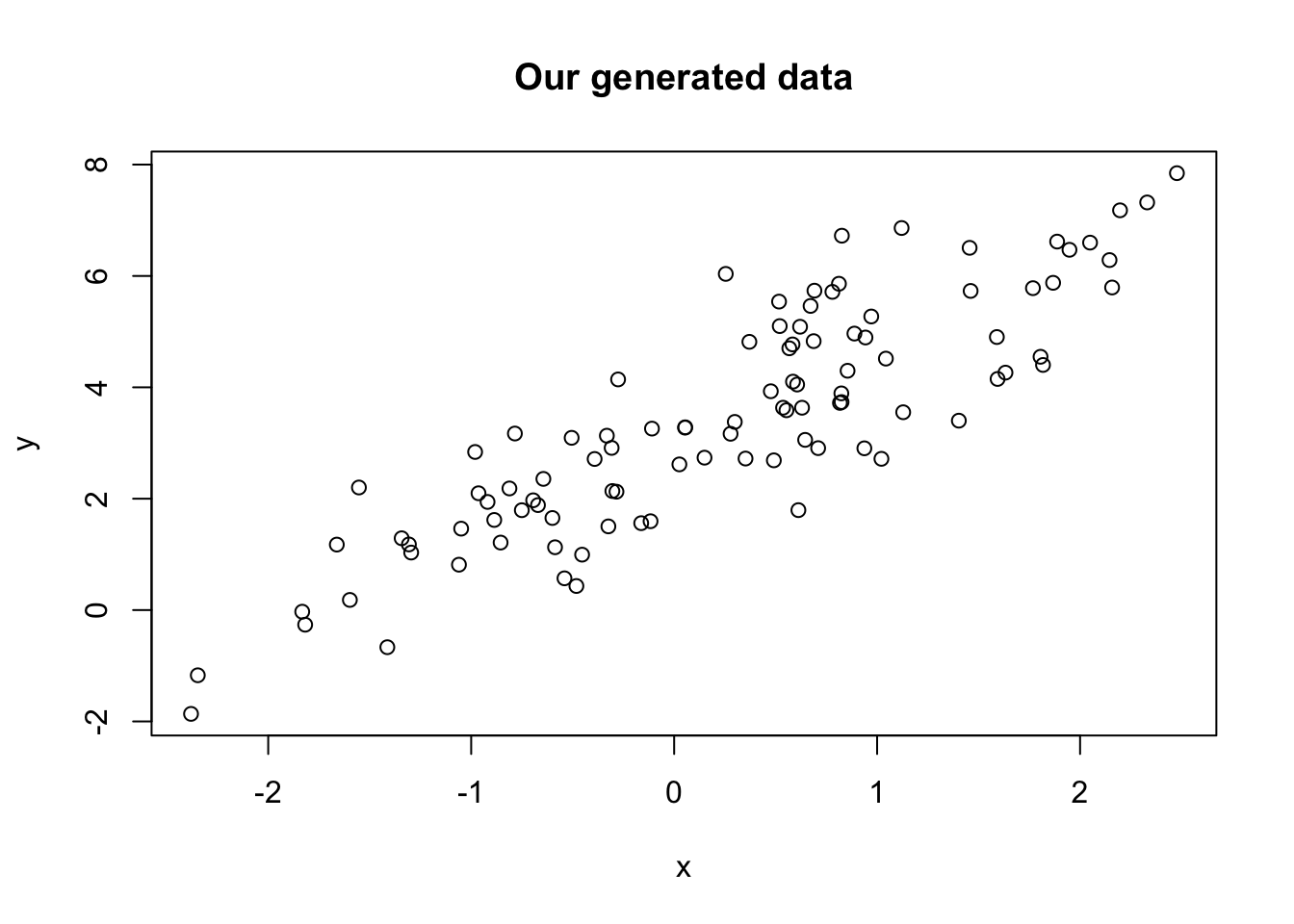

Now, let’s run our regressions

# Run b_ols with and intercept
b_ols(data = the_data, y_var = "y", X_vars = "x", intercept = T)

##                  y
## intercept 1.594535
## x         3.022053

b_ols(data = the_data, y_var = "y", X_vars = "x", intercept = F)

##         y
## x 2.16881

Notice that T and TRUE are identical in R—as are F and FALSE.

Let’s check our regressions with R’s canned function felm() (from the lfe package). Notice that you can specify a regression without an intercept using -1 in the regression formula:⁵

library(lfe)
# With an intercept:
felm(y ~ x, data = the_data) %>% summary()
## 
## Call:
##    felm(formula = y ~ x, data = the_data) 
## 
## Residuals:
##      Min       1Q   Median       3Q      Max 
## -2.20347 -0.60278 -0.01114  0.61898  2.60970 
## 
## Coefficients:
##             Estimate Std. Error t value Pr(>|t|)    
## (Intercept)  3.02205    0.10353   29.19   <2e-16 ***
## x            1.59454    0.09114   17.50   <2e-16 ***
## ---
## Signif. codes:  0 '***' 0.001 '**' 0.01 '*' 0.05 '.' 0.1 ' ' 1
## 
## Residual standard error: 1.011 on 98 degrees of freedom
## Multiple R-squared(full model): 0.7575   Adjusted R-squared: 0.755 
## Multiple R-squared(proj model): 0.7575   Adjusted R-squared: 0.755 
## F-statistic(full model):306.1 on 1 and 98 DF, p-value: < 2.2e-16 
## F-statistic(proj model): 306.1 on 1 and 98 DF, p-value: < 2.2e-16
# Without an intercept:
felm(y ~ x - 1, data = the_data) %>% summary()
## 
## Call:
##    felm(formula = y ~ x - 1, data = the_data) 
## 
## Residuals:
##    Min     1Q Median     3Q    Max 
## 0.3592 2.0732 2.8736 3.7755 5.5697 
## 
## Coefficients:
##   Estimate Std. Error t value Pr(>|t|)    
## x   2.1688     0.2757   7.867 4.62e-12 ***
## ---
## Signif. codes:  0 '***' 0.001 '**' 0.01 '*' 0.05 '.' 0.1 ' ' 1
## 
## Residual standard error: 3.132 on 99 degrees of freedom
## Multiple R-squared(full model): -1.351   Adjusted R-squared: -1.375 
## Multiple R-squared(proj model): -1.351   Adjusted R-squared: -1.375 
## F-statistic(full model):-56.89 on 1 and 99 DF, p-value: 1 
## F-statistic(proj model): 61.89 on 1 and 99 DF, p-value: 4.62e-12

Finally, let’s compare the two sets of predictions graphically:⁶

# The estimates
b_w <- b_ols(data = the_data, y_var = "y", X_vars = "x", intercept = T)
b_wo <- b_ols(data = the_data, y_var = "y", X_vars = "x", intercept = F)
# Plot the points
plot(
  # The variables for the plot
  x = the_data$x, y = the_data$y,
  # Labels and title
  xlab = "x", ylab = "y", main = "Our generated data")
# Plot the line from the 'with intercept' regression in yellow
abline(a = b_w[1], b = b_w[2], col = "lightblue", lwd = 3)
# Plot the line from the 'without intercept' regression in purple
abline(a = 0, b = b_w[1], col = "purple4", lwd = 2)
# Add a legend
legend(x = min(the_data$x), y = max(the_data$y),
  legend = c("with intercept", "w/o intercept"),
  # Line widths
  lwd = c(3, 2),
  # Colors
  col = c("lightblue", "purple4"),
  # No box around the legend
  bty = "n")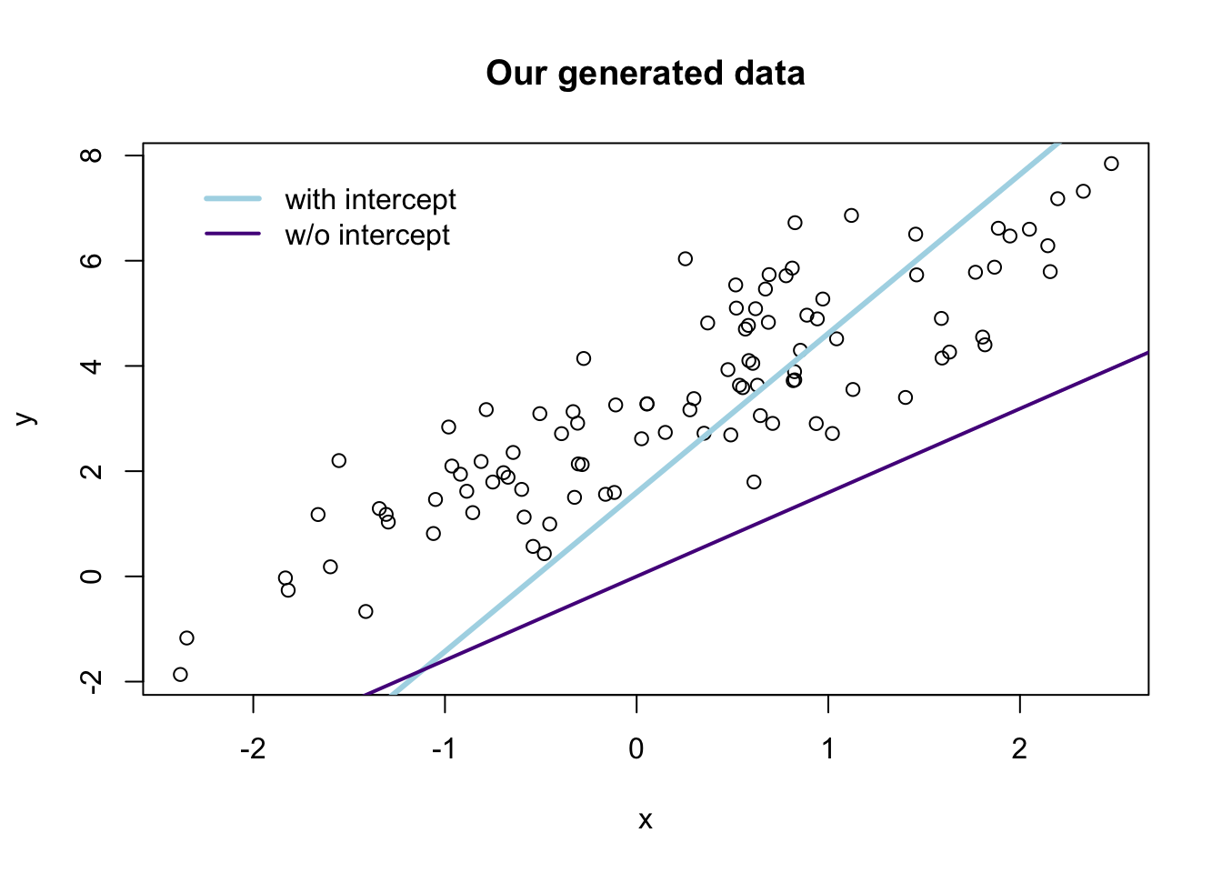

FWL theorem

As mentioned above, we are going to dive into the Frisch-Waugh-Lovell (FWL) theorem.

Setting up

First, load a few packages and the ever-popular automobile dataset.

# Setup ----
# Options
options(stringsAsFactors = F)
# Load the packages
library(dplyr)
library(lfe)
library(readr)
library(MASS)
# Set the working directory
setwd("/Users/edwardarubin/Dropbox/Teaching/ARE212/Spring2017/Section04/")
# Load the dataset from CSV
cars <- read_csv("auto.csv")

Next, because we often want to convert a tbl_df, tibble, or data.frame to a matrix, after selecting a few columns, let’s create function for this task. The function will accept:

data: a dataset
vars: a vector of the name or names of variables that we want inside our matrix

Write the function:

to_matrix <- function(the_df, vars) {
  # Create a matrix from variables in var
  new_mat <- the_df %>%
    # Select the columns given in 'vars'
    select_(.dots = vars) %>%
    # Convert to matrix
    as.matrix()
  # Return 'new_mat'
  return(new_mat)
}

Now incorporate the function in the b_ols() function from above. This addition will really clean up the function.

b_ols <- function(data, y_var, X_vars, intercept = TRUE) {
  # Require the 'dplyr' package
  require(dplyr)
  # Create the y matrix
  y <- to_matrix(the_df = data, vars = y_var)
  # Create the X matrix
  X <- to_matrix(the_df = data, vars = X_vars)
  # If 'intercept' is TRUE, then add a column of ones
  if (intercept == T) {
    # Bind a column of ones to X
    X <- cbind(1, X)
    # Name the new column "intercept"
    colnames(X) <- c("intercept", X_vars)
  }
  # Calculate beta hat
  beta_hat <- solve(t(X) %*% X) %*% t(X) %*% y
  # Return beta_hat
  return(beta_hat)
}

Does it work?

b_ols(the_data, y_var = "y", X_vars = "x", intercept = T)

##                  y
## intercept 3.022053
## x         1.594535

b_ols(the_data, y_var = "y", X_vars = "x", intercept = F)

##         y
## x 2.16881

Yes!

The theorem

The first few times I saw the Frisch-Waugh-Lovell theorem in practice, I did not appreciate it. However, I’ve become a pretty big fan of it—FWL is helpful in a number of ways.⁷ The theorem can give you some interesting insights into what is going on inside of OLS, how to interpret coefficients, and how to implement really messy regressions. We will focus on the first two points today….

Recall that for an arbitrary regression

\[ \mathbf{y} = \mathbf{X}_1 \beta_1 + \mathbf{X}_2 \beta_2 + \boldsymbol{\varepsilon} \]

FWL tells us that we can estimate \(\beta_1\) with \(\mathbf{b}_1\) using

\[ \mathbf{b}_1 = \left(\mathbf{X}_1'\mathbf{X}_1\right)^{-1}\mathbf{X}_1'\mathbf{y} - \left(\mathbf{X}_1'\mathbf{X}_1\right)^{-1}\mathbf{X}_1'\mathbf{X}_2 \mathbf{b}_2 \]

Now define \(\mathbf{M}_2\) as the residual-maker matrix, such that post-multiplying \(\mathbf{M}_2\) by another matrix \(\mathbf{C}\) (i.e., \(\mathbf{M}_2\mathbf{C}\)) will yield the residuals from regressing \(\mathbf{C}\) onto \(\mathbf{X}_2\).

Further, define \(\mathbf{X}_1^\ast = \mathbf{M}_2\mathbf{X}_1\) and \(\mathbf{y}^\ast = \mathbf{M}_2\mathbf{y}\). These starred matrices are the respective matrices residualized on \(\mathbf{X}_2\) (regressing the matrices on \(\mathbf{X}_2\) and calculating the residuals).

FWL tells us that we can write the estimate of \(\beta_1\) as

\[ \mathbf{b}_1 = \left(\mathbf{X}_1^{\ast\prime}\mathbf{X}_1^{\ast}\right)^{-1}\mathbf{X}_1^{\ast\prime}\mathbf{y}^{\ast}\]

What does this expression tell us? We can recover the estimate for \(\beta_1\) (\(\mathbf{b}_1\)) by

running a regression of \(\mathbf{y}\) on \(\mathbf{X}_1\) and subtracting off an “adjustment”, or
running a regression of a residualized \(\mathbf{y}\) on a residualized \(\mathbf{X}_1\).

The same procedure works for calculating \(\mathbf{b}_2\). Max’s course notes show the full derivation for FWL.

In practice

The first insight of FWL is that FWL generates the same estimate for \(\beta_1\) as the standard OLS estimator \(\mathbf{b}\) (for the equation)

\[ \mathbf{y} = \mathbf{X}_1 \beta_1 + \mathbf{X}_2 \beta_2 + \boldsymbol{\varepsilon} \]

The “algorithm” for estimating \(\beta_1\) via FWL is

Regress \(\mathbf{y}\) on \(\mathbf{X}_2\).
Save the residuals. Call them \(\mathbf{e}_{\mathbf{y}\mathbf{X}_2}\).
Regress \(\mathbf{X}_1\) on \(\mathbf{X}_2\).
Save the residuals. Call them \(\mathbf{e}_{\mathbf{X}_1\mathbf{X}_2}\).
Regress \(\mathbf{e}_{\mathbf{y}\mathbf{X}_2}\) on \(\mathbf{e}_{\mathbf{X}_1\mathbf{X}_2}\).

You have to admit it is pretty impressive… or at least slightly surprising.

Just in case you don’t believe me/FWL, let’s implement this algorithm using our trusty b_ols() function, regressing price on mileage and weight (with an intercept).

Before we run any regressions, we should write a function that produces the residuals for a given regression. I will keep the same syntax (arguments) as the b_ols() and will name the function resid_ols(). Within the function, we will create the \(\mathbf{X}\) and \(\mathbf{y}\) matrices just as we do in b_ols(), and then we will use the residual-maker matrix \[ \mathbf{I}_n - \mathbf{X} \left(\mathbf{X}^\prime \mathbf{X}\right)^{-1} \mathbf{X}^\prime \] which we post-multiply by \(\mathbf{y}\) to get the residuals from regressing \(\mathbf{y}\) on \(\mathbf{X}\).

resid_ols <- function(data, y_var, X_vars, intercept = TRUE) {
  # Require the 'dplyr' package
  require(dplyr)
  # Create the y matrix
  y <- to_matrix(the_df = data, vars = y_var)
  # Create the X matrix
  X <- to_matrix(the_df = data, vars = X_vars)
  # If 'intercept' is TRUE, then add a column of ones
  if (intercept == T) {
    # Bind a column of ones to X
    X <- cbind(1, X)
    # Name the new column "intercept"
    colnames(X) <- c("intercept", X_vars)
  }
  # Calculate the sample size, n
  n <- nrow(X)
  # Calculate the residuals
  resids <- (diag(n) - X %*% solve(t(X) %*% X) %*% t(X)) %*% y
  # Return 'resids'
  return(resids)
}

Now, let’s follow the steps above (note that we can combine steps 1 and 2, since we have a function that takes residuals—likewise with steps 3 and 4).

# Steps 1 and 2: Residualize 'price' on 'weight' and an intercept
e_yx <- resid_ols(data = cars, y_var = "price",
  X_vars = "weight", intercept = T)
# Steps 3 and 4: Residualize 'mpg' on 'weight' and an intercept
e_xx <- resid_ols(data = cars, y_var = "mpg",
  X_vars = "weight", intercept = T)
# Combine the two sets of residuals into a data.frame
e_df <- data.frame(e_yx = e_yx[,1], e_xx = e_xx[,1])
# Step 5: Regress e_yx on e_xx without an intercept
b_ols(data = e_df, y_var = "e_yx",
  X_vars = "e_xx", intercept = F)

##           e_yx
## e_xx -49.51222

Finally, the standard OLS estimator—no residualization magic—to check our work:

b_ols(data = cars, y_var = "price", X_vars = c("mpg", "weight"))

##                 price
## intercept 1946.068668
## mpg        -49.512221
## weight       1.746559

Boom. There you have it: FWL in action. And it works.

So what does this result reveal? I would say one key takeaway is that when we have multiple covariates (a.k.a. independent variables), the coefficient on variable \(x_k\) represents the relationship between \(y\) and \(x_k\) after controlling for the other covariates.

Another reason FWL is such a powerful result is for computational purposes: if you have a huge dataset with many observations and many variables, but you only care about the coefficients on a few variables (e.g., the case of individual fixed effects), then you can make use of FWL. Residualize the outcome variable and the covariates of interest on the covariates you do not care about. Then complete FWL. This process allows you to invert smaller matrices. Recall that you are inverting \(\mathbf{X}^{\prime}\mathbf{X}\), which means that the more variables you have, more larger the matrix you must invert. Matrix inversion is computationally intense,⁸ so by reducing the number of variables in any given regression, you can reduce the computational resources necessary for your (awesome) regressions. R’s felm() and Stata’s reghdfe take advantage of this result (though they do something a bit different in practice, to speed things up even more).

Omitted variable bias

Before we move on from FWL, let’s return to an equation we breezed past above: \[ \mathbf{b}_1 = \left(\mathbf{X}_1'\mathbf{X}_1\right)^{-1}\mathbf{X}_1'\mathbf{y} - \left(\mathbf{X}_1'\mathbf{X}_1\right)^{-1}\mathbf{X}_1'\mathbf{X}_2 \mathbf{b}_2 \]

What does this equation tell us? We can recover the OLS estimate for \(\beta_1\) by regressing \(\mathbf{y}\) on \(\mathbf{X}_1\), minus an adjustment equal to \(\left(\mathbf{X}_1'\mathbf{X}_1\right)^{-1}\mathbf{X}_1'\mathbf{X}_2 \mathbf{b}_2\).

Orthogonal covariates

Notice that if \(\mathbf{X}_1\) and \(\mathbf{X}_2\) are orthogonal (\(\mathbf{X}_1^\prime\mathbf{X}_2 = \mathbf{0}\)), then the adjustment goes to zero. The FWL interpretation for this observation is that residualizing \(\mathbf{X}_1\) on \(\mathbf{X}_2\)—when the two matrices are orthogonal—will return \(\mathbf{X}_1\).

Let’s confirm in R.

First, we generate another dataset.

# Set the seed
set.seed(12345)
# Set the sample size
n <- 1e5
# Generate x1, x2, and error from ind. N(0,1)
the_data <- tibble(
  x1 = rnorm(n),
  x2 = rnorm(n),
  e = rnorm(n))
# Calculate y = 1.5 x1 + 3 x2 + e
the_data <- mutate(the_data,
  y = 1.5 * x1 + 3 * x2 + e)

First run the regression of y on x1—omitting x2. Then run the regression of y on x1 and x2.

# Regression omitting 'x2'
b_ols(the_data, y_var = "y", X_vars = "x1", intercept = F)

##          y
## x1 1.50369

# Regression including 'x2'
b_ols(the_data, y_var = "y", X_vars = c("x1", "x2"), intercept = F)

##           y
## x1 1.501565
## x2 3.002701

Pretty good. Our variables x1 and x2 are not perfectly orthogonal, so the adjustment is not exactly zero—but it is very small.

Correlated covariates

Return to the equation once more…. \[ \mathbf{b}_1 = \left(\mathbf{X}_1'\mathbf{X}_1\right)^{-1}\mathbf{X}_1'\mathbf{y} - \left(\mathbf{X}_1'\mathbf{X}_1\right)^{-1}\mathbf{X}_1'\mathbf{X}_2 \mathbf{b}_2 \]

We’ve already talked about the case where \(\mathbf{X}_1\) and \(\mathbf{X_2}\) are orthogonal. Let’s now think about the case where they are not orthogonal.

The first observation to make is that the adjustment is now non-zero. What does a non-zero adjustment mean? In practice, it means that our results will differ—perhaps considerably—depending on whether we include or exclude the other covariates.

Let’s see this case in action (in R).

We need to generate another dataset, but this one needs \(x_1\) and \(x_2\) to be correlated (removing one of the I’s from I.I.D. normal). Specifically, we will generate two variables \(x_1\) and \(x_2\) from a multivariate normal distribution—allowing correlation between the variables. The MASS package offers the mvrnorm() function⁹ for generating random variables from a multivariate normal distribution. To use the mvrnorm() function, we need to create a variance-covariance matrix for our variables. I’m going with a variance-covariance matrix with ones on the diagonal and 0.95 on the off-diagonal elements.¹⁰ Finally, we will feed the mvrnorm() function a two-element vector of means (into the argument mu), which tells the function our desired means for each of the variables it will generate (\(x_1\) and \(x_2\)). Finally, the data-generating process (DGP) for our \(y\) will be \[ \mathbf{y} = \mathbf{1} + 2 \mathbf{x}_1 + 3 \mathbf{x}_2 + \boldsymbol{\varepsilon} \]

# Load the MASS package
library(MASS)
# Create a var-covar matrix
v_cov <- matrix(data = c(1, 0.95, 0.95, 1), nrow = 2)
# Create the means vector
means <- c(5, 10)
# Define our sample size
n <- 1e5
# Set the seed
set.seed(12345)
# Generate x1 and x2
X <- mvrnorm(n = n, mu = means, Sigma = v_cov, empirical = T)
# Create a tibble for our data, add generate error from N(0,1)
the_data <- tbl_df(X) %>% mutate(e = rnorm(n))
# Set the names
names(the_data) <- c("x1", "x2", "e")
# The data-generating process
the_data <- the_data %>% mutate(y = 1 + 2 * x1 + 3 * x2 + e)

Now that we have the data, we will run three regressions:

y regressed on an intercept, x1, and x2
y regressed on an intercept and x1
y regressed on an intercept and x2

# Regression 1: y on int, x1, and x2
b_ols(the_data, y_var = "y", X_vars = c("x1", "x2"), intercept = T)

##                  y
## intercept 1.012006
## x1        1.995968
## x2        3.000975

# Regression 2: y on int and x1
b_ols(the_data, y_var = "y", X_vars = "x1", intercept = T)

##                   y
## intercept 16.767124
## x1         4.846894

# Regression 3: y on int and x2
b_ols(the_data, y_var = "y", X_vars = "x2", intercept = T)

##                   y
## intercept -7.969850
## x2         4.897144

So what do we see here?

First, the regression that matches the true data-generating process produces coefficient estimates that are pretty much spot on (we have a fairly large sample).

Second, omitting one of the \(x\) variables really messes up the coefficient estimate on the other variable. This “messing up” is what economists omitted variable bias. What’s going on? Look back at the “adjustment” we discussed above: by omitting one of the variables—say \(\mathbf{x}_2\)—from our regression, we are omitting the adjustment. In other words: if there is a part (variable) of the data-generating process that you do not model, and the omitted variable is is correlated with a part that you do model, you are going to get the wrong answer.

This result should make you at least a little uncomfortable. What about all those regressions you see in papers? How do we know there isn’t an omitted variable lurking in the background, biasing the results?¹¹

Bad controls

Let’s take one more lesson from FWL: what happens when we add variables to the regression that (1) are not part of the DGP, and (2) are correlated with variables in the DGP?¹²

We will generate the data in a way similar to what we did above for omitted variable bias,¹³ but we will omit \(x_2\) from the data-generating process. \[ \mathbf{y} = \mathbf{1} + 2 \mathbf{x}_1 + \boldsymbol{\varepsilon} \]

# Create a var-covar matrix
v_cov <- matrix(data = c(1, 1 - 1e-6, 1 - 1e-6, 1), nrow = 2)
# Create the means vector
means <- c(5, 5)
# Define our sample size
n <- 1e5
# Set the seed
set.seed(12345)
# Generate x1 and x2
X <- mvrnorm(n = n, mu = means, Sigma = v_cov, empirical = T)
# Create a tibble for our data, add generate error from N(0,1)
the_data <- tbl_df(X) %>% mutate(e = rnorm(n))
# Set the names
names(the_data) <- c("x1", "x2", "e")
# The data-generating process
the_data <- the_data %>% mutate(y = 1 + 2 * x1 + e)

Now we will run three more regressions:

y regressed on an intercept and x1 (the DGP)
y regressed on an intercept, x1, and x2
y regressed on an intercept and x2

# Regression 1: y on int and x1 (DGP)
b_ols(the_data, y_var = "y", X_vars = "x1", intercept = T)

##                  y
## intercept 1.016691
## x1        1.996981

# Regression 2: y on int, x1, and x2
b_ols(the_data, y_var = "y", X_vars = c("x1", "x2"), intercept = T)

##                   y
## intercept 1.0166882
## x1        1.4387198
## x2        0.5582615

# Regression 3: y on int and x2
b_ols(the_data, y_var = "y", X_vars = "x2", intercept = T)

##                  y
## intercept 1.016695
## x2        1.996980

What’s going on here? The regression that matches the true DGP yields the correct coefficient estimates, but when we add \(x_2\) as a control, thinks start getting crazy. FWL helps us think about the problem here: the because \(x_1\) and \(x_2\) are so strongly correlated,¹⁴ when we “control for” \(x_2\), we remove meaningful variation—misattributing some of \(x_1\)’s variation to \(x_2\). If you are in the game of prediction, this result is not really an issue. If you are in the game of inference on the coefficients, then this result should be further reason for caution.

The R\(^2\) family

As you’ve discussed in lecture and seen in your homework, R² is a very common measure of it. The three types of R² you will most often see are

Uncentered R² (\(R^2_\text{uc}\)) measures how much of the variance in the data is explained by our model (inclusive of the intercept), relative to predicting \(\mathbf{y} = 0\).
Centered R² (plain old \(R^2\)) measures how much of the variance in the data is explained by our model, relative to predicting \(\mathbf{y}=\bar y\).
Adjusted R² (\(\bar{R}^2\)) applies a penalty to the centered R² for adding covariates to the model.

Formal definitions

We can write down the formal mathematical definitions for each of the types of R². We are going to assume the model has an intercept.

Uncentered R²

\[ R^2_\text{uc} = \dfrac{\hat{\mathbf{y}}^\prime \hat{\mathbf{y}}}{\mathbf{y}^\prime \mathbf{y}} = 1 - \dfrac{\mathbf{e}^\prime \mathbf{e}}{\mathbf{y}^\prime \mathbf{y}} = 1 - \dfrac{\sum_i (y_i - \hat{y}_i)^2}{\sum_i (y_i - 0)^2} = 1 - \dfrac{\text{SSR}}{\text{SST}_0} \] where \(SST_0\) is the total sum of squares relative to zero—this notation is a bit different from Max’s notes.

Centered R²

The formula is quite similar, but we are now demeaning by \(\bar{y}\) instead of zero: \[ R^2 = 1 - \dfrac{\mathbf{e}^\prime \mathbf{e}}{\mathbf{y}^{\ast\prime} \mathbf{y}^{\ast}} = 1 - \dfrac{\sum_i (y_i - \hat{y}_i)^2}{\sum_i (y_i - \bar{y})^2} = 1 - \dfrac{\text{SSR}}{\text{SST}} = \dfrac{\text{SSM}}{\text{SST}} \] where \(SST\) is the (standard definition of) total sum of squares, and \(\mathbf{y}^{\ast}\) denotes the demeaned vector of \(\mathbf{y}\).

Adjusted R²

\[ \bar{R}^2 = 1 - \dfrac{n-1}{n-k}\left(1-R^2\right) \] where \(n\) is the number of observations and \(k\) is the number of covariates.

R\(^2\) in R

We’ve covered the intuition and mathematics behind R², let’s now apply what we know by calculating the three measures of R² in R. We’ll use the data in auto.csv (loaded above as cars).

It will be helpful to have a function that creates the demeaning matrix \(\mathbf{A}\). Recall from Max’s notes that \(\mathbf{A}\) is defined as \[ \mathbf{A} = \mathbf{I}_n - \left(\dfrac{1}{n}\right)\mathbf{i}\mathbf{i}^\prime \] where \(\mathbf{i}\) is an \(n\)-by-\(1\) vectors of ones. When \(\mathbf{A}\) is post-multiplied by an arbitrary \(n\)-by-\(k\) matrix \(\mathbf{Z}\) (e.g., \(\mathbf{A}\mathbf{Z}\)) the result is an \(n\)-by-\(k\) matrix whose columns are the demeaned columns of \(\mathbf{Z}\).

The function will accept \(N\), the desired number of rows.

# Function that demeans the columns of Z
demeaner <- function(N) {
  # Create an N-by-1 column of 1s
  i <- matrix(data = 1, nrow = N)
  # Create the demeaning matrix
  A <- diag(N) - (1/N) * i %*% t(i)
  # Return A
  return(A)
}

Now let’s write a function that spits out three values of R² we discussed above when we feed it the same inputs as our b_ols() function.¹⁵ We will make use of a few functions from above: to_matrx(), resid_ols(), demeaner()

# Start the function
r2_ols <- function(data, y_var, X_vars) {
  # Create y and X matrices
  y <- to_matrix(data, vars = y_var)
  X <- to_matrix(data, vars = X_vars)
  # Add intercept column to X
  X <- cbind(1, X)
  # Find N and K (dimensions of X)
  N <- nrow(X)
  K <- ncol(X)
  # Calculate the OLS residuals
  e <- resid_ols(data, y_var, X_vars)
  # Calculate the y_star (demeaned y)
  y_star <- demeaner(N) %*% y
  # Calculate r-squared values
  r2_uc  <- 1 - t(e) %*% e / (t(y) %*% y)
  r2     <- 1 - t(e) %*% e / (t(y_star) %*% y_star)
  r2_adj <- 1 - (N-1) / (N-K) * (1 - r2)
  # Return a vector of the r-squared measures
  return(c("r2_uc" = r2_uc, "r2" = r2, "r2_adj" = r2_adj))
}

And now we run the function and check it with felm()’s output

# Our r-squared function
r2_ols(data = cars, y_var = "price", X_vars = c("mpg", "weight"))

##     r2_uc        r2    r2_adj 
## 0.8698475 0.2933891 0.2734846

# Using 'felm'
felm(price ~ mpg + weight, cars) %>% summary()

## 
## Call:
##    felm(formula = price ~ mpg + weight, data = cars) 
## 
## Residuals:
##    Min     1Q Median     3Q    Max 
##  -3332  -1858   -504   1256   7507 
## 
## Coefficients:
##              Estimate Std. Error t value Pr(>|t|)   
## (Intercept) 1946.0687  3597.0496   0.541  0.59019   
## mpg          -49.5122    86.1560  -0.575  0.56732   
## weight         1.7466     0.6414   2.723  0.00813 **
## ---
## Signif. codes:  0 '***' 0.001 '**' 0.01 '*' 0.05 '.' 0.1 ' ' 1
## 
## Residual standard error: 2514 on 71 degrees of freedom
## Multiple R-squared(full model): 0.2934   Adjusted R-squared: 0.2735 
## Multiple R-squared(proj model): 0.2934   Adjusted R-squared: 0.2735 
## F-statistic(full model):14.74 on 2 and 71 DF, p-value: 4.425e-06 
## F-statistic(proj model): 14.74 on 2 and 71 DF, p-value: 4.425e-06

I’ll leave the regression-without-an-intercept fun to you.

Overfitting

R² is often used to measure the fit of your model. So why does Max keep telling you that maximal R² isn’t a very good goal?¹⁶ The short answer: overfitting.

If you have enough variables, you can probably find a way to fit your outcome variable pretty well,¹⁷ but it doesn’t actually mean you are going to be able to predict any better outside of your sample or that you are learning anything valuable about the data-generating process.

As an aside, let’s imagine we want to use dplyr’s select() function now. Try select(cars, rep78) in your console. What happens? If you loaded MASS after dplyr, MASS has covered up dplyr’s select() function with its own—you may have noticed a message that said The following object is masked from `package:dplyr`: select. You can specify that you want dplyr’s function using the syntax dplyr::select(). We will use this functionality below.

To see this idea in practice, let’s add 50 random variables to the cars dataset (and drop the rep78 and make variables).

# Find the number of observations in cars
n <- nrow(cars)
# Fill an n-by-50 matrix with random numbers from N(0,1)
set.seed(12345)
rand_mat <- matrix(data = rnorm(n * 50, sd = 10), ncol = 50)
# Convert rand_mat to tbl_df
rand_df <- tbl_df(rand_mat)
# Change names to x1 to x50
names(rand_df) <- paste0("x", 1:50)
# Bind cars and rand_df; convert to tbl_df; call it 'cars_rand'
cars_rand <- cbind(cars, rand_df) %>% tbl_df()
# Drop the variable 'rep78' (it has NAs)
cars_rand <- dplyr::select(cars_rand, -rep78, -make)

Now we are going to use the function lapply() (covered near the end of last section) to progressively add variables to a regression where price is the outcome variable (there will always be an intercept).

result_df <- lapply(
  X = 2:ncol(cars_rand),
  FUN = function(k) {
    # Apply the 'r2_ols' function to columns 2:k
    r2_df <- r2_ols(
      data = cars_rand,
      y_var = "price",
      X_vars = names(cars_rand)[2:k]) %>%
      matrix(ncol = 3) %>% tbl_df()
    # Set names
    names(r2_df) <- c("r2_uc", "r2", "r2_adj")
    # Add a column for k
    r2_df$k <- k
    # Return r2_df
    return(r2_df)
  }) %>% bind_rows()

Let’s visualize R² and adjusted R² as we include more variables.

# Plot unadjusted r-squared
plot(x = result_df$k, y = result_df$r2,
  type = "l", lwd = 3, col = "lightblue",
  xlab = expression(paste("k: number of columns in ", bold("X"))),
  ylab = expression('R' ^ 2))
# Plot adjusted r-squared
lines(x = result_df$k, y = result_df$r2_adj,
  type = "l", lwd = 2, col = "purple4")
# The legend
legend(x = 0, y = max(result_df$r2),
  legend = c(expression('R' ^ 2),
    expression('Adjusted R' ^ 2)),
  # Line widths
  lwd = c(3, 2),
  # Colors
  col = c("lightblue", "purple4"),
  # No box around the legend
  bty = "n")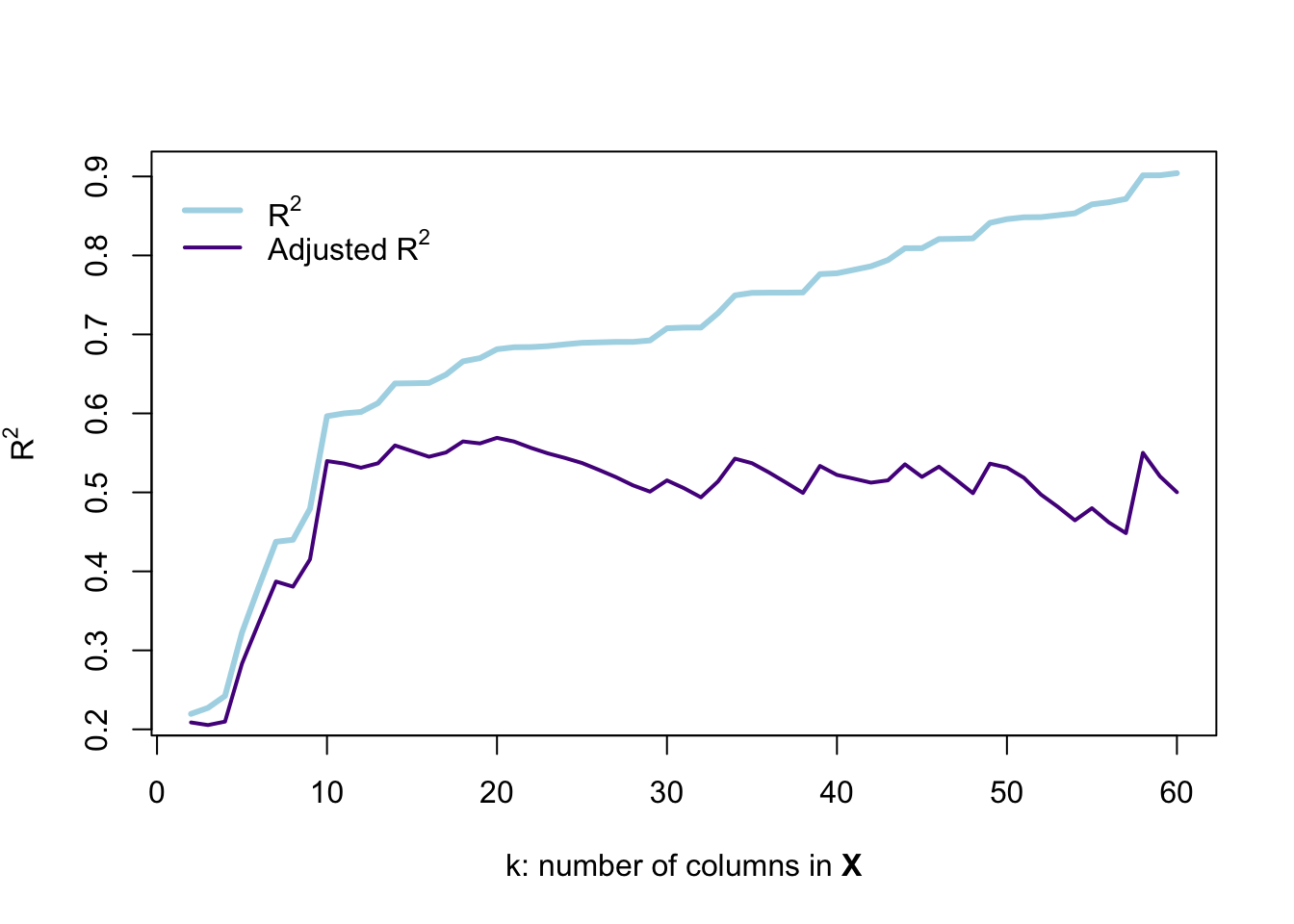

This figure demonstrates why R² is not a perfect descriptor for model fit: as we add variables that are pure noise, R² describes the fit as actually getting substantially better—every variable after the tenth column in \(\mathbf{X}\) is randomly generated and surely has nothing to do with the price of a car. However, R² continues to increase… and even the adjusted R² doesn’t really give us a clear picture that the model is falling apart.

If you are interested in a challenge, change the r2_ols() function so that it also spits out AIC and SIC and then re-run this simulation. You should find something like:

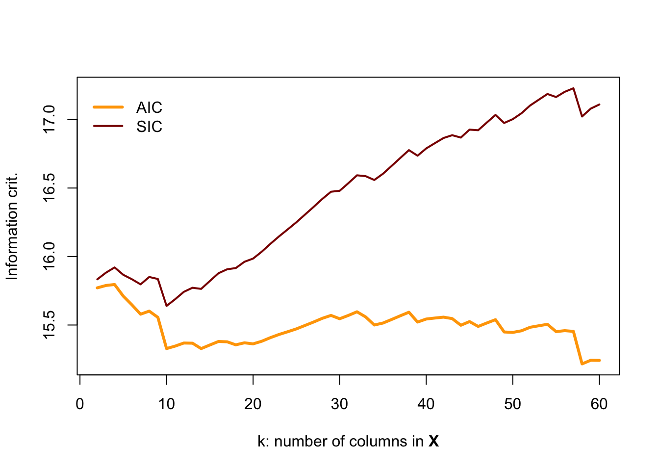
Here, BIC appears to do the best job noticing when the data become poor.

Sorry for starting with the wrong way to break up a line of code.↩
?read_csv, assuming you have the readr package loaded.↩
You will also notice that the file name that we feed to the function is read as the file argument. You can get the same result by typing read_csv("my_file.csv") or read_csv(file = "my_file.csv").↩
I changed the names of the arguments in our function to be a bit more descriptive and easy to use.↩
Correspondingly, you can force an intercept using +1 in the regression formula.↩
See here for help with color names in R. You can also use html color codes.↩
I googled “frisch waugh lovell fan club” but did not find anything: you should consider starting something formal.↩
At least that is what I hear…↩
Akin to the univariate random normal generator rnorm().↩
We need a 2-by-2 variance-covariance matrix because we have two variables and thus need to specify the variance for each (the diagonal elements) and the covariance between the two variables.↩
This class is not focused on causal inference—ARE 213 covers that topic—but it is still worth keeping omitted variable bias in mind, no matter which course you take.↩
In some sense, this case is the opposite of omitted variable bias.↩
I’m going to increase the covariance and set the means of \(x_1\) and \(x_2\) equal.↩
The collinearity of the two covariates is another problem.↩
I will assume intercept is always TRUE and thus will omit it.↩
in econometrics and in life↩
Remember the spurious correlation website Max showed you?↩

Section 4: FWL and model fit