Admin

Change in office hours this week: 10:30am–12pm in Giannini 236. (Apologies for the inconvenience; department-level scheduling issues…)

What you will need

Packages:

Previously used: dplyr and haven
New: lfe

Data: The auto.dta file.

Summary of last time

In Section 2, we covered the data structures of vectors and matrices.

Follow up: Numeric vs. double

Someone asked about double versus numeric. It turns out that numeric is a more general class/mode. Numeric objects come in different modes. Specifically, numeric objects can be either double-precision or integer (single-precision is not really an option in R, unless you are calling C or Fortran at a lower level).

In practice:

# Does as.numeric() create integers or doubles?
is.double(as.numeric(1))
## [1] TRUE
is.integer(as.numeric(1))
## [1] FALSE
# Are integers and doubles numeric?
is.numeric(as.double(1))
## [1] TRUE
is.numeric(as.integer(1))
## [1] TRUE

Follow up: Vectorized operations

I want to point out that I probably did not give vectors a fair shake. While seemingly simple, R allows you to do a lot of things with vectors that might be much more difficult in other languages. Specifically, R allows you to apply (most) functions to vectors, rather than individual elements of a vector.

For an underwhelming example, if you want to square each number in a vector vec in R, you can simply write vec^2. The alternative that many languages use requires iterating through the vector and squaring the individual elements while simultaneously storing the results.

# Define the vector
vec <- 1:5
# Square the elements of the vector
vec2 <- vec^2
# Look at the result
vec2
## [1]  1  4  9 16 25

Summary of this section

This section covers functions, loops, and some simulation. We will take what you have been covering in lecture—the ordinary least squares (OLS) estimator—and create our very own OLS function.¹ Then we will play around with our OLS function.

Cleaning up

You will occasionally need to clear up some space for memory in R (or just tidy up your environment). To see the objects you are currently storing in memory, you can either (1) look in the “Environment” pane of RStudio or (2) use the ls() function (the function does not need any inputs).

If you decide to clean up, the function rm() is your friend. Here are three uses:

# Remove a single object from memory
rm(item1)
# Remove to (or more) objects from memory
rm(list = c("item2", "item3"))
# Remove everything from memory
rm(list = ls())

You also can use the garbage control (gc()) function if you’ve loaded and removed several large datasets. It is not the same as rm(); gc() has more to do with space allocated for objects than the space actually used.²

Custom functions

Up to this point, we have written some lines of R code that rely upon already-defined functions. We are now going to try writing our own function.

There are a few reasons why you want to write your own function:

Max forbids you from doing your homeworks with the canned functions.
You have a task for which there is not a function.
You have a task that needs to be repeated, and you do not want to keep writing the same \(N\) lines of code over and over again.

More simply: if you need to do the same task more than twice, you should probably write a function for that task, rather than copying and pasting the code dozens of times.

Custom function basics

To write a custom function in R, you use a function named function().³ The specific syntax for defining a function looks like

foo <- function(arg1, arg2) {
  ...
  return(final_stuff)
}

which says that we are defining a new function named foo that takes the arguments arg1 and arg2 (your function can take as many or as few arguments as you like). The function then completes some tasks (you would have actual code where you currently see ...), and then the function returns a value of final_stuff using the return() function.⁴ Notice that after you define the function’s arguments, you open a curly bracket and immediately start a new line. You end function’s definition by closing the curly bracket (on a line by itself).

For a quick example of a custom function, let’s define a function that accepts three arguments and returns the product of the three arguments.

# Define the function (named 'triple_prod')
triple_prod <- function(x, y, z) {
  # Take the product of the three arguments
  tmp_prod <- x * y * z
  # Return 'tmp_prod'
  return(tmp_prod)
}

# Test the function
triple_prod(x = 2, y = 3, z = 5)
## [1] 30

An OLS function

As discussed above, functions are very helpful when you have a task that you want to repeat many times. In this class,⁵ you will estimate \(\widehat{\boldsymbol{\beta}}_{ols}\) many times. So let’s write a function that calculates the OLS estimator for \(\boldsymbol{\beta}\).

Recall that for an outcome (dependent) variable \(\mathbf{y}\) and a matrix of independent variables \(\mathbf{X}\) (including a column of ones for the intercept), the OLS estimator for \(\boldsymbol{\beta}\) in the equation

\[ \mathbf{y} = \mathbf{X} \boldsymbol{\beta} + \boldsymbol{\varepsilon} \]

\[ \widehat{\boldsymbol{\beta}}_{ols} = \left(\mathbf{X}'\mathbf{X}\right)^{-1}\mathbf{X}'\mathbf{y} \]

Part of writing a function is determining what you want and do not want the function to do. You have a lot of options. Should it accept matrices, tibbles, data frames, etc.? Should the function automatically add a row for the interept? Should it calculate the R² or only \(\widehat{\boldsymbol{\beta}}_{ols}\)? …

For now, let’s assume the function will accept a tibble with the variables that we want for both \(\mathbf{y}\) and \(\mathbf{X}\). And let’s name the function b_ols. In addition to the tibble (let’s pass the tibble to the function through the argument data), the function will probably need (at least) two more arguments: y and X, which will be the name of the dependent variable and the names of the independent variables, respectively. Finally—for now—let’s say the function will only return the OLS estimate for \(\boldsymbol{\beta}\).

The function should thus look something like

b_ols <- function(data, y, X) {
  # Put some code here...
  return(beta_hat)
}

Aside: Load your data

Our OLS function will need some data. Load the auto.dta data from Section 1 (also in this section’s zip file). (Remember: you will need the haven package to load the .dta file.) We’re not loading the data inside our function because we’ll probably want to use the function on different datasets.

# Setup ----
# Options
options(stringsAsFactors = F)
# Packages
library(haven)
## Warning: package 'haven' was built under R version 3.4.3
library(dplyr)
# Set the directory
setwd("/Users/edwardarubin/Dropbox/Teaching/ARE212/Spring2017/Section03/")

# Load the data ----
cars <- read_dta(file = "auto.dta")

`require`d packages

Spoiler: Our function is going to make use of the dplyr package. So let’s tell our function to make sure the dplyr package is loaded. The function require() is the standard way to have a function make sure a package is loaded. You use it just like the library() function. Since we know that we plan to use the dplyr package, let’s require it within our function:

b_ols <- function(data, y, X) {
  # Require the 'dplyr' package
  require(dplyr)
  # Put some code here...
  return(beta_hat)
}

`select_`ing variables

Let’s take an inventory of which objects we have, once we are inside the function. We have data, which is a tibble with columns that represent various variables. We have y, the name of our outcome variable (e.g., weight). And we have X, a vector of the names of our independent variables (e.g. c("mpg", "weight")).⁶

The first step for our function is to grab the data for y and X from data. For this task, we will use a variation of the select() function introduced in Section 1: select_(). The difference between select() and select_() (besides the underscore) is that select() wants the variable names without quotes (non-standard evaluation), e.g. select(cars, mpg, weight). This notation is pretty convenient except when you are writing your own function. Generally, you will have variable/column names in a character vector, and select(cars, "mpg", "weight") does not work. Here is where select_() comes in: it wants you to use characters (standard evaluation). There is one more complexity: while select_(cars, "mpg", "weight") works, select_(cars, c("mpg", "weight")) does not. So if you have a vector of variable names, like our X, you need a slightly different way to use select_(). The solution is the .dots argument in select_(): select_(cars, .dots = c("mpg", "weight")) works!

So… we now want to select the y and X variables from data. Let’s do it.

# Select y variable data from 'data'
y_data <- select_(data, .dots = y)
# Select X variable data from 'data'
X_data <- select_(data, .dots = X)

This code should do the trick. To test it, you’ll need to define y and X (e.g., y = "price" and X = c("mpg", "weight")).

Exercise: Finish the function

The function now looks like

b_ols <- function(data, y, X) {
  # Require the 'dplyr' package
  require(dplyr)
  # Select y variable data from 'data'
  y_data <- select_(data, .dots = y)
  # Select X variable data from 'data'
  X_data <- select_(data, .dots = X)
  # Put some code here...
  return(beta_hat)
}

Fill in the # Put some code here... section of our new function with the code needed to produce OLS estimates via matrix operations. More kudos for fewer lines.

Hints/reminders:

The data objects y_data and X_data are still tibbles. You eventually want matrices.
Don’t forget the intercept.
If you finish early, adapt the function to return centered R², uncentered R², and adjusted R².

Matrices

We have a few tasks left:

Add an intercept (column of ones) to X_data
Convert the data objects to matrices
Calculate \(\widehat{\boldsymbol{\beta}}_{ols}\) via matrix operations

First, let’s add a column of ones to X_data. We will use mutate_().⁷ The mutate() and mutate_() functions allow us to add new columns/variables to an existing data object. Often the new variables will be a combination of existing variables, but in our case, we just want a column of ones, so all we need to do is write mutate_(X_data, "ones" = 1).

It is customary to have the intercept column be the first column in the matrix. We can use select_() again to change the order of the columns: select_(X_data, "ones", .dots = X).

We will use the as.matrix() function to convert our tibbles to matrices.

Finally, once we have our matrices, we can use the basic matrix functions discussed in Section 2—namely %*%, t(), and solve()—to calculate \(\widehat{\boldsymbol{\beta}}_{ols} = \left(\mathbf{X}'\mathbf{X}\right)^{-1}\mathbf{X}'\mathbf{y}\).

Putting these steps together, we can finish our function:

b_ols <- function(data, y, X) {
  # Require the 'dplyr' package
  require(dplyr)

  # Select y variable data from 'data'
  y_data <- select_(data, .dots = y)
  # Convert y_data to matrices
  y_data <- as.matrix(y_data)

  # Select X variable data from 'data'
  X_data <- select_(data, .dots = X)
  # Add a column of ones to X_data
  X_data <- mutate_(X_data, "ones" = 1)
  # Move the intercept column to the front
  X_data <- select_(X_data, "ones", .dots = X)
  # Convert X_data to matrices
  X_data <- as.matrix(X_data)

  # Calculate beta hat
  beta_hat <- solve(t(X_data) %*% X_data) %*% t(X_data) %*% y_data
  # Change the name of 'ones' to 'intercept'
  rownames(beta_hat) <- c("intercept", X)
  # Return beta_hat
  return(beta_hat)
}

Piping

Our OLS function is nice, but we redefined y_data and X_data a number of times. There’s nothing wrong with these intermediate steps, but dplyr provides a fantastic tool %>% for bypassing these steps to clean up your code. The operator is known as the pipe or chain command.⁸

The way the pipe (%>%) works is by taking the output from one expression and plugging it into the next expression (defaulting to the first argument in the second expression). For example, rather than writing the two lines of code

# Select the variables
tmp_data <- select(cars, price, mpg, weight)
# Summarize the selected variables
summary(tmp_data)
##      price            mpg            weight    
##  Min.   : 3291   Min.   :12.00   Min.   :1760  
##  1st Qu.: 4220   1st Qu.:18.00   1st Qu.:2250  
##  Median : 5006   Median :20.00   Median :3190  
##  Mean   : 6165   Mean   :21.30   Mean   :3019  
##  3rd Qu.: 6332   3rd Qu.:24.75   3rd Qu.:3600  
##  Max.   :15906   Max.   :41.00   Max.   :4840

we can do it in a single line (and without creating the unnecessary object tmp_data)

cars %>% select(price, mpg, weight) %>% summary()
##      price            mpg            weight    
##  Min.   : 3291   Min.   :12.00   Min.   :1760  
##  1st Qu.: 4220   1st Qu.:18.00   1st Qu.:2250  
##  Median : 5006   Median :20.00   Median :3190  
##  Mean   : 6165   Mean   :21.30   Mean   :3019  
##  3rd Qu.: 6332   3rd Qu.:24.75   3rd Qu.:3600  
##  Max.   :15906   Max.   :41.00   Max.   :4840

What is going on here? We’re plugging cars into the first argument of the select() expression, and then plugging the output from select() into summary(). If you want to save the result from the last expression (summary() here), use the normal method, e.g.

some_summaries <- cars %>% select(price, mpg, weight) %>% summary()

If it helps you remember what a pipe is doing, you can use a period with a comma:⁹

# Four equivalent expressions
cars %>% select(price, mpg) %>% summary()
cars %>% select(., price, mpg) %>% summary()
select(cars, price, mpg) %>% summary()
summary(select(cars, price, mpg))

You can see that pipes also help you avoid situations with crazy parentheses.

Now let’s apply these pipes to the OLS function above. Essentially any time you redefine an object, you could have used a pipe. Also note that pipes can extend to the next line and are uninterrupted by comments.

b_ols <- function(data, y, X) {
  # Require the 'dplyr' package
  require(dplyr)

  # Create the y matrix
  y_data <- data %>%
    # Select y variable data from 'data'
    select_(.dots = y) %>%
    # Convert y_data to matrices
    as.matrix()

  # Create the X matrix
  X_data <- data %>%
    # Select X variable data from 'data'
    select_(.dots = X) %>%
    # Add a column of ones to X_data
    mutate_("ones" = 1) %>%
    # Move the intercept column to the front
    select_("ones", .dots = X) %>%
    # Convert X_data to matrices
    as.matrix()

  # Calculate beta hat
  beta_hat <- solve(t(X_data) %*% X_data) %*% t(X_data) %*% y_data
  # Change the name of 'ones' to 'intercept'
  rownames(beta_hat) <- c("intercept", X)
  # Return beta_hat
  return(beta_hat)
}

Quality check

Let’s check our function’s results against one of R’s canned regression functions. The base installation of R provides the function lm(), which works great. However, we are going to use the felm() function from the lfe package. The felm() function has some nice benefits over lm() that you will probably want at some point, namely the ability to deal with many fixed effects, instrumental variables, and multi-way clustered errors. (Don’t worry if you do not know what that last sentence meant. You will soon.)

Install the lfe package.

install.packages("lfe")

Load it.

library(lfe)

Run the relevant regression with felm():¹⁰

# Run the regression with 'felm'
canned_ols <- felm(formula = price ~ mpg + weight, data = cars)
# Summary of the regression
canned_ols %>% summary()
## 
## Call:
##    felm(formula = price ~ mpg + weight, data = cars) 
## 
## Residuals:
##    Min     1Q Median     3Q    Max 
##  -3332  -1858   -504   1256   7507 
## 
## Coefficients:
##              Estimate Std. Error t value Pr(>|t|)   
## (Intercept) 1946.0687  3597.0496   0.541  0.59019   
## mpg          -49.5122    86.1560  -0.575  0.56732   
## weight         1.7466     0.6414   2.723  0.00813 **
## ---
## Signif. codes:  0 '***' 0.001 '**' 0.01 '*' 0.05 '.' 0.1 ' ' 1
## 
## Residual standard error: 2514 on 71 degrees of freedom
## Multiple R-squared(full model): 0.2934   Adjusted R-squared: 0.2735 
## Multiple R-squared(proj model): 0.2934   Adjusted R-squared: 0.2735 
## F-statistic(full model):14.74 on 2 and 71 DF, p-value: 4.425e-06 
## F-statistic(proj model): 14.74 on 2 and 71 DF, p-value: 4.425e-06

Run the regression with our function b_ols():

b_ols(data = cars, y = "price", X = c("mpg", "weight"))
##                 price
## intercept  -49.512221
## mpg          1.746559
## weight    1946.068668

They match!

Loops

Loops are a very common programming tool. Just like functions, loops help us with repetitive tasks.

`for()` loops

for loops are classic. You give the program a list and then tell it to do something with each of the objects in the list. R’s power with vectors obviates some uses of for loops, but there are still many cases in which you will need some type of loop. You will also hear people say that for loops are a bad idea in R. Don’t entirely believe them. There are cases where you can do things much faster with other types of loops—particularly if you are going to parallelize and have access to a lot of computing resources—but for loops can still be very helpful.

In R, the for loop has the following structure

for (i in vec) {
  # Complex computations go here
}

Example of an actual (simple) for loop:

for (i in 1:5) {
  print(paste("Hi", i))
}

## [1] "Hi 1"
## [1] "Hi 2"
## [1] "Hi 3"
## [1] "Hi 4"
## [1] "Hi 5"

A final note on for loops in R: R keeps the last iteration’s values in memory. This behavior can help with troubleshooting, but it can also sometimes lead to confusion.

While for loops are great, we’re going to focus on a different type of loop today…

`lapply()`

The lapply() function is part of a family of apply() functions in R (apply(), lapply(), sapply(), mapply(), etc.). Each function takes slightly different inputs and/or generates slightly different outputs, but the idea is generally the same. And the idea if very similar to that of a loop: you give lapply() a list or vector X and a function FUN, and lapply() with then apply the function FUN to each of the elements in X. lapply() returns a list¹¹ of the results generated by FUN for each of the elements of X.

Finally, it is worth noting that lapply() sticks the elements of X into the first argument of the function FUN (you can still define other arguments of FUN) in a way very similar to the pipe operator (%>%).

Here is a simplistic example of lapply():

lapply(X = 0:4, FUN = sqrt)

## [[1]]
## [1] 0
## 
## [[2]]
## [1] 1
## 
## [[3]]
## [1] 1.414214
## 
## [[4]]
## [1] 1.732051
## 
## [[5]]
## [1] 2

Notice the slightly different notation of the list, relative to the vectors we previously discussed.

Unlike for loops, nothing done inside of an lapply() call is kept in memory after the function finishes (aside from the final results, if you assign them to an object).

`lapply()` meets `b_ols()`

What if we want to regress each of the numerical variables in the cars data on mpg and weight (with the exception of rep78, because I don’t really understand what “Repair Record 1978” means)? Surprise, surprise: we can use lapply().

What should our X value be? The numeric variables excluding rep78, mpg, and weight. Let’s create a vector for it.

target_vars <- c("price", "headroom", "trunk", "length", "turn",
  "displacement", "gear_ratio", "foreign")

With respect to the FUN argument, keep in mind that lapply() plugs the X values into the first argument of the function. For b_ols(), the first argument is data, which is not what we currently want to vary. We want to vary y, which is the second argument. Rather than redefining the b_ols() function, we can augment it by wrapping another function around it. For example,

function(i) b_ols(data = cars, y = i, X = c("mpg", "weight"))

This line of code creates a new, unnamed function with one argument i. The argument i is then fed to our b_ols() function as its y argument. Let’s put it all together…

# The 'lapply' call
results_list <- lapply(
  X = target_vars,
  FUN = function(i) b_ols(data = cars, y = i, X = c("mpg", "weight"))
  )
# The results
results_list

## [[1]]
##                 price
## intercept  -49.512221
## mpg          1.746559
## weight    1946.068668
## 
## [[2]]
##                headroom
## intercept -0.0098904309
## mpg        0.0004668253
## weight     1.7943225731
## 
## [[3]]
##                  trunk
## intercept -0.082739270
## mpg        0.003202433
## weight     5.849262628
## 
## [[4]]
##                 length
## intercept  -0.35546594
## mpg         0.02496695
## weight    120.11619444
## 
## [[5]]
##                   turn
## intercept -0.059092537
## mpg        0.004498541
## weight    27.323996368
## 
## [[6]]
##           displacement
## intercept    0.7604918
## mpg          0.1103151
## weight    -151.9910285
## 
## [[7]]
##              gear_ratio
## intercept  0.0007521123
## mpg       -0.0004412382
## weight     4.3311476331
## 
## [[8]]
##                 foreign
## intercept -0.0194295266
## mpg       -0.0004677698
## weight     2.1235056112

These results are a bit of a mess. Let’s change the list into a more legible data structure. We will use lapply() to apply the function data.frame() to each of the results (each of the elements of results_list). Finally, we will use the bind_cols() function from dplyr to bind all of the results together (so we don’t end up with another list).¹²

# Cleaning up the results list
results_df <- lapply(X = results_list, FUN = data.frame) %>% bind_cols()
# We lose the row names in the process; add them back
rownames(results_df) <- c("intercept", "mpg", "weight")
# Check out results_df
results_df

##                 price      headroom        trunk       length         turn
## intercept  -49.512221 -0.0098904309 -0.082739270  -0.35546594 -0.059092537
## mpg          1.746559  0.0004668253  0.003202433   0.02496695  0.004498541
## weight    1946.068668  1.7943225731  5.849262628 120.11619444 27.323996368
##           displacement    gear_ratio       foreign
## intercept    0.7604918  0.0007521123 -0.0194295266
## mpg          0.1103151 -0.0004412382 -0.0004677698
## weight    -151.9910285  4.3311476331  2.1235056112

Exercise: Check your work

Check the results in results_df using lapply() and felm(). Hint: remember to check the class of the object returned felm(). You might want to try the coef() function on the object returned by felm().

Simulation

One of the main reasons to learn the apply() family of functions is that they are very flexible (and easily parallelized).¹³ This flexibility lends them to use in simulation, which basically means we want to generate random numbers and to test/observe properties of estimators. And repeat many times.

Examining bias in one sample

We often examine the (finite-sample) properties of estimators through simulation.

Let’s start with a function that generates some data, estimates coefficients via OLS, and calculates the bias.

# A function to calculate bias
data_baker <- function(sample_n, true_beta) {
  # First generate x from N(0,1)
  x <- rnorm(sample_n)
  # Now the error from N(0,1)
  e <- rnorm(sample_n)
  # Now combine true_beta, x, and e to get y
  y <- true_beta[1] + true_beta[2] * x + e
  # Define the data matrix of independent vars.
  X <- cbind(1, x)
  # Force y to be a matrix
  y <- matrix(y, ncol = 1)
  # Calculate the OLS estimates
  b_ols <- solve(t(X) %*% X) %*% t(X) %*% y
  # Convert b_ols to vector
  b_ols <- b_ols %>% as.vector()
  # Calculate bias, force to 2x1 data.frame()
  the_bias <- (true_beta - b_ols) %>%
    matrix(ncol = 2) %>% data.frame()
  # Set names
  names(the_bias) <- c("bias_intercept", "bias_x")
  # Return the bias
  return(the_bias)
}

This function will calculate the bias of the OLS estimator for a single sample,

# Set seed
set.seed(12345)
# Run once
data_baker(sample_n = 100, true_beta = c(1, 3))

##   bias_intercept      bias_x
## 1    -0.02205339 -0.09453503

Examining bias in many samples

But what if you want to run 10,000 simulations? Should you just copy and paste 10,000 times? Probably not.¹⁴ Use lapply() (or replicate()). And let’s write one more function wrapped around data_baker().

# A function to run the simulation
bias_simulator <- function(n_sims, sample_n, true_beta) {

  # A function to calculate bias
  data_baker <- function(sample_n, true_beta) {
    # First generate x from N(0,1)
    x <- rnorm(sample_n)
    # Now the error from N(0,1)
    e <- rnorm(sample_n)
    # Now combine true_beta, x, and e to get y
    y <- true_beta[1] + true_beta[2] * x + e
    # Define the data matrix of independent vars.
    X <- cbind(1, x)
    # Force y to be a matrix
    y <- matrix(y, ncol = 1)
    # Calculate the OLS estimates
    b_ols <- solve(t(X) %*% X) %*% t(X) %*% y
    # Convert b_ols to vector
    b_ols <- b_ols %>% as.vector()
    # Calculate bias, force to 2x1 data.frame()
    the_bias <- (true_beta - b_ols) %>%
      matrix(ncol = 2) %>% data.frame()
    # Set names
    names(the_bias) <- c("bias_intercept", "bias_x")
    # Return the bias
    return(the_bias)
  }

  # Run data_baker() n_sims times with given parameters
  sims_dt <- lapply(
    X = 1:n_sims,
    FUN = function(i) data_baker(sample_n, true_beta)) %>%
    # Bind the rows together to output a nice data.frame
    bind_rows()

  # Return sim_dt
  return(sims_dt)
}

To run the simulation 10,000 times, use the code (can take a little while):

# Set seed
set.seed(12345)
# Run it
sim_dt <- bias_simulator(n_sims = 1e4, sample_n = 100, true_beta = c(1,3))
# Check the results with a histogram
hist(sim_dt[,2],
  breaks = 30,
  main = "Is OLS unbiased?",
  xlab = "Bias")
# Emphasize the zero line
abline(v = 0, col = "blue", lwd = 3)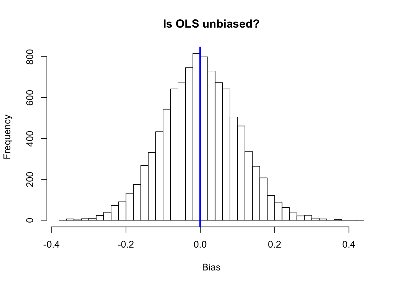

In section 5 we’ll talk about parallelization, which can greatly reduce the time of your simulations.

Extensions/challenges

How few characters can you use to write a function that estimates coefficients via OLS? Can you keep this function parsimonious while expanding its flexibility (allowing it to take different data structures with and without intercepts)?
Can you find any speed/efficiency improvements over my data_baker() and bias_simulator() functions? Feel free to include parallelization.
How would you generate vectors of two random variables that are correlated (i.e. \(x\) and \(\varepsilon\) are not independent)? Does this correlation affect anything in your bias simulations?

Max has probably mentioned that you have to write your own functions in this class. While relying upon the canned R functions is prohibited, you can use them to check your work.↩
Sorry if this garbage control function is not clear: I’m not a computer scientist.↩
So meta, right?↩
You can get away with not using the return() function, but it is generally thought of as bad form.↩
not to mention the life of an empirical economist↩
I guess I’ve asserted these definitions of y and X. You’re free to do whatever you like.↩
You could use mutate() too.↩
See the package magrittr for even more pipe operators.↩
Note: the period will actually allow you to shift the argument to which the prior expression’s output is sent.↩
felm(), like most regression functions I’ve seen in R, uses a formula where the dependent variable¹⁰ is separated from the independent variables with a tilde (~).↩
This is our first time meeting a list. Lists are yet another way to store data in R—like vectors, matrices, data.frames, and tibbles. You can create lists with the list() function much like you create vectors with the c() function: my_list <- list("a", 1, c(1,2,3)). Lists differ in that they do not require a uniform data type, as demonstrated in the list in the preceding sentence. Lists also utilize a slightly different indexing: you access the third element of the list my_list via my_list[[3]]. Notice the extra set of square brackets.↩
We could alternatively try sapply(), which attempts to return nicely formatted objects. However, you never know if it is going to succeed in nicely formatting your results. If it doesn’t, then it returns a list. This sort of inconsistency is not very helpful in programming, so I generally avoid sapply().↩
Parallelization basically means that you run things at the same time—instead of waiting until one thing finishes to start the next. Thus some tasks can be parallelized—simulations for unbiased estimators—while other tasks that depend upon the output from previous iterations are more difficult to parallelize. We’ll talk more about parallelization in section 5.↩
Definitely not.↩

Section 3: Functions and loops