What you will need

Working and up-to-date installations of R and RStudio
Data files “auto.csv” and “auto.dta”. Download a zipped folder here.
An internet connection
Optional: A healthy source of caffeine

Summary

In this section we will dive into R. We start by installing and loading three useful packages (dplyr, haven, and readr). We then load two datasets and begin summarizing and manipulating them. Finally, we’ll make our first plots.

Packages in R

Open RStudio.¹

While the base R installation helpful/powerful, R’s true potential comes from combining combining the core installation with its many packages generated through collaboration (see CRAN’s list of packages ²).

Installing packages

Now, let’s install a few packages that will prove useful this semester…

# Install the package named "dplyr"
install.packages("dplyr")
# Install the packages named "haven" and "readr"
install.packages(c("haven", "readr"))

A few things to notice here:

The name of the function install.packages() is plural regardless of the number of packages.
Each package’s name is surrounded by quotes (e.g. "haven"). These quotation marks are how R knows the difference between characters/strings and objects (objects hold values). R generally does not care whether you use single quote ('') or double quotes (""), but you should be consistent.
We can create a vector of packages using the combine function c(). Example: c(1, 2, 3) is a three-element vector whose elements are 1, 2, and 3. Similarly, c("haven", "readr") is a two-element vector whose elements are the "haven" and "readr". Vectors are a big deal in R.
The hashtag (#) is the symbol that creates comments in R.

Loading packages

To check that the installations were successful, we will load the packages that we installed above.

R uses the library() function to load a package (we give the name of the package as the argument to the function).³

library(dplyr)

## 
## Attaching package: 'dplyr'

## The following objects are masked from 'package:stats':
## 
##     filter, lag

## The following objects are masked from 'package:base':
## 
##     intersect, setdiff, setequal, union

library(haven)

## Warning: package 'haven' was built under R version 3.4.3

library(readr)

Notice that we did not need to call the packages with quotations around their names (though it would still work).

Loading data

Loading a dataset in R requires three things:

The path of the data file (where the data exist on your computer)
The name of the data file
The proper function for the type of dataset (e.g. we use different functions for .csv and .dta files)

File paths

R wants file paths as character vectors (i.e. the file path surrounded by quotations). For example, "/Users/edwardarubin/Dropbox/Teaching/ARE212" is the path to my folder for this course (on my computer).⁴ ⁵

To change the directory in R, use the setwd(). For instance, to change R’s directory to my course folder

setwd("/Users/edwardarubin/Dropbox/Teaching/ARE212")

To find R’s current working directory, simply type getwd():

getwd()

## [1] "/Users/edwardarubin/Dropbox/Teaching/ARE212/Spring2017"

There are a few ways to deal with file paths and directories. One common way is to use setwd() at the top of your script (or invoke the function whenever you need to change directories).

I find clearer to store the paths that I will use—at the start of my R script, I define the paths relevant to the files I use within the script. I prefer this method because it allows me to quickly update paths and easily access subfolders.

# The path to my ARE 212 folder (ARE212)
dir_class <- "/Users/edwardarubin/Dropbox/Teaching/ARE212/"
# The path to my section 1 folder (Section01), which is inside my ARE 212 folder
dir_section1 <- paste0(dir_class, "Section01/")

Notice the use of the paste0() function here: we paste together the value of the object dir_class and the string "Section01". The function paste0(), by default, pastes without any spaces in between the objects. The function paste() defaults to including a single space (you can feed the functions additional parameters to change these behaviors).

As a quick example:

# Default use of paste0()
paste0(1, 2, 3)

## [1] "123"

# Default use of paste()
paste(1, 2, 3)

## [1] "1 2 3"

# Setting the separation parameter to " " (the default)
paste(1, 2, 3, sep = " ")

## [1] "1 2 3"

# Changing the separation parameter to "+"
paste(1, 2, 3, sep = "+")

## [1] "1+2+3"

Finally, notice that RStudio assists you with completing file paths (begin typing and press tab). This completion can be super useful.

`dir()`

The function dir() allows you to see contents of a folder. dir() can help when you forget the name of the file you want. To see the contents of a folder, give the folder’s file path to dir():

# Look inside my ARE212 folder (dir_class stores the path)
dir(dir_class)

##  [1] "_site.yml"             "analyticstracking.php"
##  [3] "contact.html"          "contact.Rmd"          
##  [5] "courseInfo.html"       "courseInfo.Rmd"       
##  [7] "footer.html"           "futureNotes.html"     
##  [9] "futureNotes.Rmd"       "htmlScript.R"         
## [11] "Images"                "index.html"           
## [13] "index.Rmd"             "LatexKnitr"           
## [15] "latexKnitr_files"      "latexKnitr.html"      
## [17] "latexKnitr.Rmd"        "notes.html"           
## [19] "notes.Rmd"             "Papers"               
## [21] "pdfScript.R"           "pdfScript.spin.R"     
## [23] "pdfScript.spin.Rmd"    "README.html"          
## [25] "README.md"             "resources.html"       
## [27] "resources.Rmd"         "Section00"            
## [29] "section00.html"        "section00.Rmd"        
## [31] "Section01"             "section01_files"      
## [33] "section01.html"        "section01.Rmd"        
## [35] "Section01.zip"         "Section02"            
## [37] "section02.html"        "section02.Rmd"        
## [39] "Section02.zip"         "Section03"            
## [41] "section03_cache"       "section03_files"      
## [43] "section03.html"        "section03.Rmd"        
## [45] "Section03.zip"         "Section04"            
## [47] "section04_cache"       "section04_files"      
## [49] "section04.html"        "section04.Rmd"        
## [51] "Section04.zip"         "Section05"            
## [53] "section05_cache"       "section05_files"      
## [55] "section05.html"        "section05.Rmd"        
## [57] "Section05.zip"         "Section06"            
## [59] "section06_cache"       "section06_files"      
## [61] "section06.html"        "section06.Rmd"        
## [63] "Section06.zip"         "Section07"            
## [65] "section07_cache"       "section07_files"      
## [67] "section07.html"        "section07.Rmd"        
## [69] "Section07.zip"         "Section08"            
## [71] "section08_cache"       "section08_files"      
## [73] "section08.html"        "section08.Rmd"        
## [75] "Section08.zip"         "Section09"            
## [77] "section09_files"       "section09.html"       
## [79] "section09.Rmd"         "Section09.zip"        
## [81] "Section10"             "section10_files"      
## [83] "section10.html"        "section10.Rmd"        
## [85] "Section10.zip"         "Section11"            
## [87] "section11_cache"       "section11_files"      
## [89] "section11.html"        "section11.Rmd"        
## [91] "site_libs"             "Spring2017"           
## [93] "syllabi.html"          "syllabi.Rmd"          
## [95] "syllabus2017.pdf"      "syllabus2018.pdf"     
## [97] "TODO.html"             "TODO.md"              
## [99] "update.bash"

# Look inside my section 1 folder (dir_section1 stores the path)
dir(dir_section1)

## [1] "auto.csv"      "auto.dta"      "README.md"     "section01.pdf"
## [5] "section01.R"

You can see there are a few files of interest in the section 1 folder—specifically, auto.csv and auto.dta.⁶

Recall that dir_section1 is an object that holds a value representing a file path, i.e.,

dir_section1

## [1] "/Users/edwardarubin/Dropbox/Teaching/ARE212/Section01/"

Notice that we get the same result if we feed dir() object’s name or its value, since R is evaluating the object:

# The object
dir(dir_section1)

## [1] "auto.csv"      "auto.dta"      "README.md"     "section01.pdf"
## [5] "section01.R"

# The object's value
dir("/Users/edwardarubin/Dropbox/Teaching/ARE212/Section01/")

## [1] "auto.csv"      "auto.dta"      "README.md"     "section01.pdf"
## [5] "section01.R"

Functions to load files

There are a lot of ways to load (data) files in R. In this class, we will mostly stick to the packages readr and haven—in addition to R’s base functions. The readr package offers functions for mostly for reading delimited data files like CSVs, TSVs, and fixed-width files. The haven package offers functions for reading data files outputted from other statistical software like Stata, SPSS (or PSPP), and SAS.

Let’s start by reading the data stored in the auto.dta file. For this task, we’ll use the read_dta() funtion from the haven package. The read_dta() function needs only one argument: the file (including the path necessary to reach the file).

Note: To learn more about a function and the arguments it accepts, you can

Press tab (in RStudio) after typing the function’s name.
Type a question mark and the function’s name into the console, e.g. ?read_dta.

Enough talk. Let’s finally load the file.

# Load the .dta file
car_data <- read_dta(paste0(dir_section1, "auto.dta"))

The <- operator is central to everything you do in R. It assigns the value(s) on the right-hand side of the arrow to the name on the left-hand side. When reading R code aloud, people often replace the arrow with “gets”. The main thing to understand is that the contents of “auto.dta” are now assigned to the name car_data. To see this, simply type the name into the console (a bad idea with really big datasets, but this dataset is not big).

car_data

## # A tibble: 74 x 12
##             make price   mpg rep78 headroom trunk weight length  turn
##            <chr> <dbl> <dbl> <dbl>    <dbl> <dbl>  <dbl>  <dbl> <dbl>
##  1   AMC Concord  4099    22     3      2.5    11   2930    186    40
##  2     AMC Pacer  4749    17     3      3.0    11   3350    173    40
##  3    AMC Spirit  3799    22    NA      3.0    12   2640    168    35
##  4 Buick Century  4816    20     3      4.5    16   3250    196    40
##  5 Buick Electra  7827    15     4      4.0    20   4080    222    43
##  6 Buick LeSabre  5788    18     3      4.0    21   3670    218    43
##  7    Buick Opel  4453    26    NA      3.0    10   2230    170    34
##  8   Buick Regal  5189    20     3      2.0    16   3280    200    42
##  9 Buick Riviera 10372    16     3      3.5    17   3880    207    43
## 10 Buick Skylark  4082    19     3      3.5    13   3400    200    42
## # ... with 64 more rows, and 3 more variables: displacement <dbl>,
## #   gear_ratio <dbl>, foreign <dbl+lbl>

If we instead had a CSV file—which we do—we could use the function read_csv() from the package readr to load the file.⁷

# Load the .csv file
car_data <- read_csv(paste0(dir_section1, "auto.csv"))

## Parsed with column specification:
## cols(
##   make = col_character(),
##   price = col_double(),
##   mpg = col_double(),
##   rep78 = col_double(),
##   headroom = col_double(),
##   trunk = col_double(),
##   weight = col_double(),
##   length = col_double(),
##   turn = col_double(),
##   displacement = col_double(),
##   gear_ratio = col_double(),
##   foreign = col_integer()
## )

# See that it looks the same as above
car_data

## # A tibble: 74 x 12
##             make price   mpg rep78 headroom trunk weight length  turn
##            <chr> <dbl> <dbl> <dbl>    <dbl> <dbl>  <dbl>  <dbl> <dbl>
##  1   AMC Concord  4099    22     3      2.5    11   2930    186    40
##  2     AMC Pacer  4749    17     3      3.0    11   3350    173    40
##  3    AMC Spirit  3799    22   NaN      3.0    12   2640    168    35
##  4 Buick Century  4816    20     3      4.5    16   3250    196    40
##  5 Buick Electra  7827    15     4      4.0    20   4080    222    43
##  6 Buick LeSabre  5788    18     3      4.0    21   3670    218    43
##  7    Buick Opel  4453    26   NaN      3.0    10   2230    170    34
##  8   Buick Regal  5189    20     3      2.0    16   3280    200    42
##  9 Buick Riviera 10372    16     3      3.5    17   3880    207    43
## 10 Buick Skylark  4082    19     3      3.5    13   3400    200    42
## # ... with 64 more rows, and 3 more variables: displacement <dbl>,
## #   gear_ratio <dbl>, foreign <int>

Note that you do not have to paste the directory onto the file name if you are already in the file’s directory (R reasonably defaults to looking in the current directory). In my case, I just need to tell R to go to the Section01 folder, where my auto.csv file lives.

read_csv("Section01/auto.csv")

## Parsed with column specification:
## cols(
##   make = col_character(),
##   price = col_double(),
##   mpg = col_double(),
##   rep78 = col_double(),
##   headroom = col_double(),
##   trunk = col_double(),
##   weight = col_double(),
##   length = col_double(),
##   turn = col_double(),
##   displacement = col_double(),
##   gear_ratio = col_double(),
##   foreign = col_integer()
## )

## # A tibble: 74 x 12
##             make price   mpg rep78 headroom trunk weight length  turn
##            <chr> <dbl> <dbl> <dbl>    <dbl> <dbl>  <dbl>  <dbl> <dbl>
##  1   AMC Concord  4099    22     3      2.5    11   2930    186    40
##  2     AMC Pacer  4749    17     3      3.0    11   3350    173    40
##  3    AMC Spirit  3799    22   NaN      3.0    12   2640    168    35
##  4 Buick Century  4816    20     3      4.5    16   3250    196    40
##  5 Buick Electra  7827    15     4      4.0    20   4080    222    43
##  6 Buick LeSabre  5788    18     3      4.0    21   3670    218    43
##  7    Buick Opel  4453    26   NaN      3.0    10   2230    170    34
##  8   Buick Regal  5189    20     3      2.0    16   3280    200    42
##  9 Buick Riviera 10372    16     3      3.5    17   3880    207    43
## 10 Buick Skylark  4082    19     3      3.5    13   3400    200    42
## # ... with 64 more rows, and 3 more variables: displacement <dbl>,
## #   gear_ratio <dbl>, foreign <int>

Playing with data

You now know how to navigate your computer and load data. You might want to do something with those data.

Exploring the data

Let’s print the data into the console again.

car_data

## # A tibble: 74 x 12
##             make price   mpg rep78 headroom trunk weight length  turn
##            <chr> <dbl> <dbl> <dbl>    <dbl> <dbl>  <dbl>  <dbl> <dbl>
##  1   AMC Concord  4099    22     3      2.5    11   2930    186    40
##  2     AMC Pacer  4749    17     3      3.0    11   3350    173    40
##  3    AMC Spirit  3799    22   NaN      3.0    12   2640    168    35
##  4 Buick Century  4816    20     3      4.5    16   3250    196    40
##  5 Buick Electra  7827    15     4      4.0    20   4080    222    43
##  6 Buick LeSabre  5788    18     3      4.0    21   3670    218    43
##  7    Buick Opel  4453    26   NaN      3.0    10   2230    170    34
##  8   Buick Regal  5189    20     3      2.0    16   3280    200    42
##  9 Buick Riviera 10372    16     3      3.5    17   3880    207    43
## 10 Buick Skylark  4082    19     3      3.5    13   3400    200    42
## # ... with 64 more rows, and 3 more variables: displacement <dbl>,
## #   gear_ratio <dbl>, foreign <int>

Not bad. We can see a few interesting things in this view of the dataset.

The dataset’s is of the class tibble (it’s like a table but with a few rules—see ?tibble::tibble).
The dataset’s dimensions are 74 by 12, meaning we have 74 rows and 12 columns.
We can also see the class of each of the columns: the make column is of “character” class, and the rest of the columns are of class “double”, with the exception of the foreign variable, which is of class “integer”.
We get a snapshot of the dataset.

What if we just want the names of the dataset? Use the names() function.

names(car_data)

##  [1] "make"         "price"        "mpg"          "rep78"       
##  [5] "headroom"     "trunk"        "weight"       "length"      
##  [9] "turn"         "displacement" "gear_ratio"   "foreign"

And what if we want to see the first six rows of the dataset? Use the head() function.

head(car_data)

## # A tibble: 6 x 12
##            make price   mpg rep78 headroom trunk weight length  turn
##           <chr> <dbl> <dbl> <dbl>    <dbl> <dbl>  <dbl>  <dbl> <dbl>
## 1   AMC Concord  4099    22     3      2.5    11   2930    186    40
## 2     AMC Pacer  4749    17     3      3.0    11   3350    173    40
## 3    AMC Spirit  3799    22   NaN      3.0    12   2640    168    35
## 4 Buick Century  4816    20     3      4.5    16   3250    196    40
## 5 Buick Electra  7827    15     4      4.0    20   4080    222    43
## 6 Buick LeSabre  5788    18     3      4.0    21   3670    218    43
## # ... with 3 more variables: displacement <dbl>, gear_ratio <dbl>,
## #   foreign <int>

What if we want to see the first 11 rows of the dataset? Use the head() function with its n argument.

head(car_data, n = 11)

## # A tibble: 11 x 12
##             make price   mpg rep78 headroom trunk weight length  turn
##            <chr> <dbl> <dbl> <dbl>    <dbl> <dbl>  <dbl>  <dbl> <dbl>
##  1   AMC Concord  4099    22     3      2.5    11   2930    186    40
##  2     AMC Pacer  4749    17     3      3.0    11   3350    173    40
##  3    AMC Spirit  3799    22   NaN      3.0    12   2640    168    35
##  4 Buick Century  4816    20     3      4.5    16   3250    196    40
##  5 Buick Electra  7827    15     4      4.0    20   4080    222    43
##  6 Buick LeSabre  5788    18     3      4.0    21   3670    218    43
##  7    Buick Opel  4453    26   NaN      3.0    10   2230    170    34
##  8   Buick Regal  5189    20     3      2.0    16   3280    200    42
##  9 Buick Riviera 10372    16     3      3.5    17   3880    207    43
## 10 Buick Skylark  4082    19     3      3.5    13   3400    200    42
## 11  Cad. Deville 11385    14     3      4.0    20   4330    221    44
## # ... with 3 more variables: displacement <dbl>, gear_ratio <dbl>,
## #   foreign <int>

And for the last 7 rows of the dataset? Use the tail() function with its n argument.

tail(car_data, n = 7)

## # A tibble: 7 x 12
##             make price   mpg rep78 headroom trunk weight length  turn
##            <chr> <dbl> <dbl> <dbl>    <dbl> <dbl>  <dbl>  <dbl> <dbl>
## 1 Toyota Corolla  3748    31     5      3.0     9   2200    165    35
## 2  Toyota Corona  5719    18     5      2.0    11   2670    175    36
## 3      VW Dasher  7140    23     4      2.5    12   2160    172    36
## 4      VW Diesel  5397    41     5      3.0    15   2040    155    35
## 5      VW Rabbit  4697    25     4      3.0    15   1930    155    35
## 6    VW Scirocco  6850    25     4      2.0    16   1990    156    36
## 7      Volvo 260 11995    17     5      2.5    14   3170    193    37
## # ... with 3 more variables: displacement <dbl>, gear_ratio <dbl>,
## #   foreign <int>

RStudio also has a nice—though sometimes slow—data viewer. You can access the data viewer through the RStudi GUI or through the View() function, e.g. View(car_data).

Summarizing the data

To make a quick summary of your dataset, you can use the summary() function.

summary(car_data)

##      make               price            mpg            rep78      
##  Length:74          Min.   : 3291   Min.   :12.00   Min.   :1.000  
##  Class :character   1st Qu.: 4220   1st Qu.:18.00   1st Qu.:3.000  
##  Mode  :character   Median : 5006   Median :20.00   Median :3.000  
##                     Mean   : 6165   Mean   :21.30   Mean   :3.406  
##                     3rd Qu.: 6332   3rd Qu.:24.75   3rd Qu.:4.000  
##                     Max.   :15906   Max.   :41.00   Max.   :5.000  
##                                                     NA's   :5      
##     headroom         trunk           weight         length     
##  Min.   :1.500   Min.   : 5.00   Min.   :1760   Min.   :142.0  
##  1st Qu.:2.500   1st Qu.:10.25   1st Qu.:2250   1st Qu.:170.0  
##  Median :3.000   Median :14.00   Median :3190   Median :192.5  
##  Mean   :2.993   Mean   :13.76   Mean   :3019   Mean   :187.9  
##  3rd Qu.:3.500   3rd Qu.:16.75   3rd Qu.:3600   3rd Qu.:203.8  
##  Max.   :5.000   Max.   :23.00   Max.   :4840   Max.   :233.0  
##                                                                
##       turn        displacement     gear_ratio       foreign      
##  Min.   :31.00   Min.   : 79.0   Min.   :2.190   Min.   :0.0000  
##  1st Qu.:36.00   1st Qu.:119.0   1st Qu.:2.730   1st Qu.:0.0000  
##  Median :40.00   Median :196.0   Median :2.955   Median :0.0000  
##  Mean   :39.65   Mean   :197.3   Mean   :3.015   Mean   :0.2973  
##  3rd Qu.:43.00   3rd Qu.:245.2   3rd Qu.:3.353   3rd Qu.:1.0000  
##  Max.   :51.00   Max.   :425.0   Max.   :3.890   Max.   :1.0000  
##

However, we often just want to know about one variable. How do you grab a single variable in R? Use the $, of course. Specifically, type the name of the dataset, followed by $, followed by the name of the variable. Again, RStudio’s autocompletion using tab is your best friend here.

To grab the price variable (named price) from the car_data dataset, we type car_data$price. And to summarize the price variable:

summary(car_data$price)

##    Min. 1st Qu.  Median    Mean 3rd Qu.    Max. 
##    3291    4220    5006    6165    6332   15906

Manipulating the data

`select()`

Now let’s move on to manipulating our dataset. The package dplyr offers a lot of help in manipulating data. dplyr is built on the paradigm of using verbs as actions on the data—for instance, select() variables and then summarize() them.

First, let’s say we only care about a subset of the variables (e.g price, mpg, weight, and length) and don’t feel like hanging on to the others. You could complete this task with R’s built-in subset() function, but let’s instead use the select() function from dplyr. All you need to do is give select() the name of the dataset (car_data) and the names of the variables that we want to keep. dplyr (and some other functions in R) uses what is called non-standard evaluation, which means you do not need to put quotes around the variable names.⁸

# Select our desired variables; define as car_sub
car_sub <- select(car_data, price, mpg, weight, length)
# Print the dataset
car_sub

## # A tibble: 74 x 4
##    price   mpg weight length
##    <dbl> <dbl>  <dbl>  <dbl>
##  1  4099    22   2930    186
##  2  4749    17   3350    173
##  3  3799    22   2640    168
##  4  4816    20   3250    196
##  5  7827    15   4080    222
##  6  5788    18   3670    218
##  7  4453    26   2230    170
##  8  5189    20   3280    200
##  9 10372    16   3880    207
## 10  4082    19   3400    200
## # ... with 64 more rows

You can see that we still have 74 rows but only four columns.

Alternatively, you can choose which variables you would like to exclude from a dataset by placing a negative sign (dash) in front of the name

select(car_data, -price, -mpg, -weight, -length)

## # A tibble: 74 x 8
##             make rep78 headroom trunk  turn displacement gear_ratio
##            <chr> <dbl>    <dbl> <dbl> <dbl>        <dbl>      <dbl>
##  1   AMC Concord     3      2.5    11    40          121       3.58
##  2     AMC Pacer     3      3.0    11    40          258       2.53
##  3    AMC Spirit   NaN      3.0    12    35          121       3.08
##  4 Buick Century     3      4.5    16    40          196       2.93
##  5 Buick Electra     4      4.0    20    43          350       2.41
##  6 Buick LeSabre     3      4.0    21    43          231       2.73
##  7    Buick Opel   NaN      3.0    10    34          304       2.87
##  8   Buick Regal     3      2.0    16    42          196       2.93
##  9 Buick Riviera     3      3.5    17    43          231       2.93
## 10 Buick Skylark     3      3.5    13    42          231       3.08
## # ... with 64 more rows, and 1 more variables: foreign <int>

`arrange()`

We often want to arrange our dataset by one or more columns. For this task, dplyr offers the arrange() function. The notation is similar to that of select: the data object’s name followed by the variables with with you would like to arrange the object. Let’s arrange by price and mpg. The second dimension of sorting here is only for demonstration (it’s pointless in the actually arrangement).

arrange(car_sub, price, mpg)

## # A tibble: 74 x 4
##    price   mpg weight length
##    <dbl> <dbl>  <dbl>  <dbl>
##  1  3291    20   2830    195
##  2  3299    29   2110    163
##  3  3667    24   2750    179
##  4  3748    31   2200    165
##  5  3798    35   2050    164
##  6  3799    22   2640    168
##  7  3829    22   2580    169
##  8  3895    26   1830    142
##  9  3955    19   3430    197
## 10  3984    30   2120    163
## # ... with 64 more rows

Having used the arrange() function on our data, what happens if we view the dataset now?

car_sub

## # A tibble: 74 x 4
##    price   mpg weight length
##    <dbl> <dbl>  <dbl>  <dbl>
##  1  4099    22   2930    186
##  2  4749    17   3350    173
##  3  3799    22   2640    168
##  4  4816    20   3250    196
##  5  7827    15   4080    222
##  6  5788    18   3670    218
##  7  4453    26   2230    170
##  8  5189    20   3280    200
##  9 10372    16   3880    207
## 10  4082    19   3400    200
## # ... with 64 more rows

It is no longer arranged. This point is important. With nearly every function in R, you must assign the output of a function to an object if you want anything to change. Otherwise, you are simply printing your results to the console.

arrange() defaults to ascending ordering; if you would like descending ordering, use the desc() function on the variables that you would like to be descending.

arrange(car_sub, desc(price), mpg)

## # A tibble: 74 x 4
##    price   mpg weight length
##    <dbl> <dbl>  <dbl>  <dbl>
##  1 15906    21   4290    204
##  2 14500    14   3900    204
##  3 13594    12   4720    230
##  4 13466    14   3830    201
##  5 12990    14   3420    192
##  6 11995    17   3170    193
##  7 11497    12   4840    233
##  8 11385    14   4330    221
##  9 10372    16   3880    207
## 10 10371    16   4030    206
## # ... with 64 more rows

`summarize()`

To create more specific summaries of your data, dplyr offers the summarize() and summarize_each() functions.⁹ These functions are really more useful when you have grouped data, but it may be helpful to first see them here in a simpler setting.

Imaging we want the mean and standard deviation of the price variable, we use the functions mean() and sd() in conjunction with summarize():

summarize(car_sub, mean(price), sd(price))

## # A tibble: 1 x 2
##   `mean(price)` `sd(price)`
##           <dbl>       <dbl>
## 1      6165.257    2949.496

You can even provide names for the newly created summaries.

summarize(car_sub, price_mean = mean(price), price_sd = sd(price))

## # A tibble: 1 x 2
##   price_mean price_sd
##        <dbl>    <dbl>
## 1   6165.257 2949.496

Because these summaries were relatively simple, we could have just typed them out…

mean(car_sub$price)

## [1] 6165.257

sd(car_sub$price)

## [1] 2949.496

Plotting the data

A final way we often play with data is by making plots. R’s default plot functions are quite simple but leave a bit to be desired with respect to aesthetics. We will cover ggplot() later in the semester, but for now, let’s make a few quick plots.

Let’s create a histogram of the cars’ milages. R’s hist() function works perfectly here. It only needs the variable of interest, but we can provide more parameters to make it pretty.

First, the plan-vanilla plot

hist(car_sub$mpg)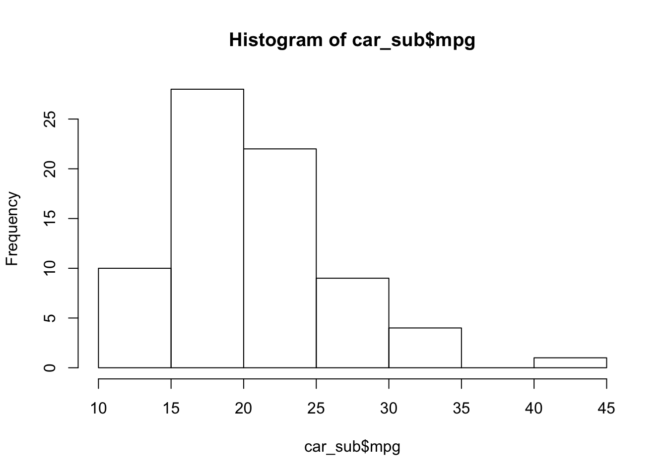

Now, a bit prettier. And let’s add a blue line for the median MPG (using the abline() function).

# The histogram function
hist(
  # The variable for the histogram
  x = car_sub$mpg,
  # The main title
  main = "Distribution of fuel economy",
  # The x-axis label
  xlab = "MPG (miles per gallon)")
# The blue vertical line at the median MPG (lwd is line width)
abline(v = median(car_sub$mpg), col = "blue", lwd = 3)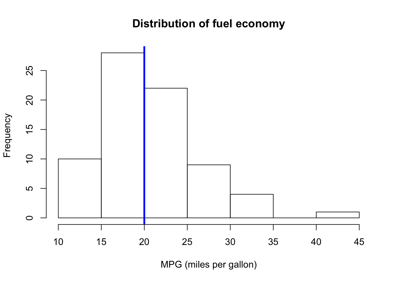

Now let’s plot price and mileage. A scatterplot will work here, and R’s base plot() function will do just fine with a scatter plot. We will give it an x variable, a y variable, and the axis titles.

plot(
  x = car_sub$mpg,
  y = car_sub$price,
  xlab = "Fuel economy (MPG)",
  ylab = "Price")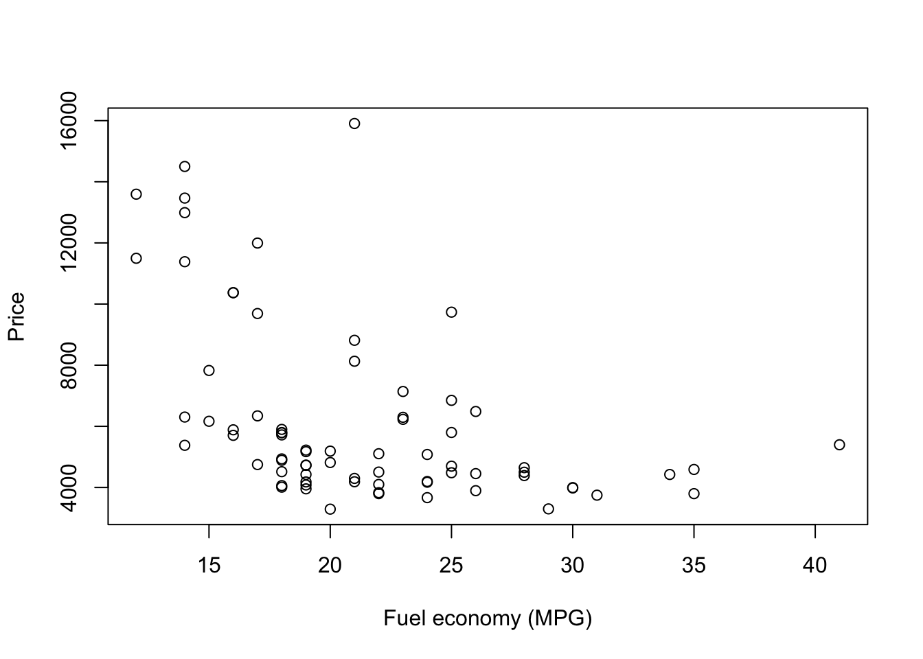

Note: I really like clearly defining the arguments of functions. And I recommend it. I find it helps keep things straight, as order matters when you are not naming each argument.

Indexing

Nearly everything in R is numerically indexed. For instance, when we create a vector of numbers, as we did earlier, each element of the vector gets a numerical index (1, 2, 3, …). You can generally access the individual elements of objects using these indexes and square brackets behind the name of the object (e.g. test[2] grabs that second element of the object test).

# Create a vector
x <- c(3, 5, 7, 9)
# Grab the second element of x
x[2]

## [1] 5

# Grab the second and third elements of x
x[c(2, 3)]

## [1] 5 7

# Grab the second and third elements of x
x[2:3]

## [1] 5 7

# See what 2:3 does
2:3

## [1] 2 3

This indexing works with data objects, as well. We just have one more dimension to consider—we have rows and columns. Rows before columns, i.e., [row, column] (but we don’t actually use the words).

To grab the first row of car_sub, we put a 1 for the row index and leave the column blank.

car_sub[1, ]

## # A tibble: 1 x 4
##   price   mpg weight length
##   <dbl> <dbl>  <dbl>  <dbl>
## 1  4099    22   2930    186

To grab the first column of car_sub, we

car_sub[, 1]

## # A tibble: 74 x 1
##    price
##    <dbl>
##  1  4099
##  2  4749
##  3  3799
##  4  4816
##  5  7827
##  6  5788
##  7  4453
##  8  5189
##  9 10372
## 10  4082
## # ... with 64 more rows

You can also use the name of a column as its index

car_sub[, "price"]

## # A tibble: 74 x 1
##    price
##    <dbl>
##  1  4099
##  2  4749
##  3  3799
##  4  4816
##  5  7827
##  6  5788
##  7  4453
##  8  5189
##  9 10372
## 10  4082
## # ... with 64 more rows

We’ll do a lot more of this indexing stuff in the future.

Linear algebra puzzles

Some classic¹⁰ R-meets-linear algebra puzzles for your enjoyment. They may use some R concepts that we have not yet covered.

Let I₅ be a 5 $\times$ 5 identity matrix. Demonstrate that I₅ is symmetric and idempotent using simple functions in R.
Generate a 2 $\times$ 2 idempotent matrix X, where X is not the identity matrix. Demonstrate that X = XX.
Generate two random variables, x and e, of dimension n = 100 such that x, e ∼ N(0, 1). Generate a random variable y according to the data generating process $y_i = x_i + e_i$. Show that if you regress y on x using the canned linear regression routine lm(), then you will get an estimate of the intercept $\beta_0$ and the coefficient on x, $\beta_1$, such that $\beta_0 = 0$ and $\beta_1 = 1$.
Show that if $\lambda_1, \lambda_2, \ldots, \lambda_5$ are the eigenvectors of a 5 $\times$ 5 matrix A, then tr(A) = $\sum_{i=1}^5 \lambda_i$.

If you do not have the most recent versions of R (3.3.2, a.k.a. Sincere Pumpkin Patch) and RStudio (1.0.136), then please check out the directions in Section 0.↩
CRAN stands for [the] Comprehensive R Archive Network↩
You can also access functions within a package without loading the whole package. Let’s say we want to load the happy() function from the fake package without loading the whole fake package. Just type fake::happy(). The double colon :: is the key here. (Note: Not all functions from a package can be accessed this way.) This method also works well when packages overlap in the names that they use for functions.↩
Windows users beware: when you copy the path from File Explorer, the slashes between folders may be in the wrong direction for R: you will need to either change the direction (from \ to /) or double them (from / to //).↩
Note: Mac (OSX) directories tend to start with “/Users/”, while Windows paths start with the name of the drive, for instance, “C:/”. If you’re using Linux, you probably don’t need my help here.↩
The files are apparently classic Stata tutorial files.↩
If you have really big delimited files (csv, tsv, fixed, width, etc.), I recommend the fread() (fast read) function from the data.table package. The whole data.table package is awesome and fast—it’s just a bit less beginner friendly than dplyr.↩
If leaving off the quotation marks makes you uncomfortable—or is actually inhibiting your programming—each dplyr function has a clone that uses standard evaluation. These standard evaluation clones have the same names as their counterparts but with an added underscore (_) at their ends (e.g. select_()).↩
If you are more comfortable with British English, you will be happy to know you can use the functions summarise() and summarise_each().↩
By classic, I mean they’ve shown up in this class’s section notes for several years.↩

Section 1: Getting started with R