Section 12: Spatial data
Admin
Announcements
- Thank you for the very sweet card!
- Next week we will wrap up spatial data and then move on to strategies for large datasets (big data), including efficient coding practices.
Last section
In our previous section we covered instrumental variables and two-state least squares—two tools an econometrician can use against the bias/inconsistency generated by omitted variable, measurement error, and simultaneous equations.
Follow up: Papers
Someone asked for a few examples of papers that apply instrumental variables. Below are several options for you. In general, it is hard to go wrong with Angrist and Krueger (or Imbens). The first two papers are actually a summary articles—the first paper has a great table of instrumental variables papers in myriad settings. The third paper (Angrist, 1990) is a classic. The fourth paper is quite new by Reed Walker (Berkeley). The fifth paper (Lee et al.) is a working paper on rural electrification by three more Berkeley folks. The last paper (Maccini and Yang, 2009) is a pretty classic paper of health, development, and measurement error.
I’ve provided the PDF of the first two papers. You’ll need to download the other papers from an IP address with access.
- Instrumental Variables and the Search for Identification: From Supply and Demand to Natural Experiments, Angrist and Krueger (2001)
- Instrumental Variables: An Econometrician’s Perspective, Imbens (2014)
- Lifetime Earnings and the Vietnam Era Draft Lottery: Evidence from Social Security Administrative Records, Angrist (1990)
- Airports, Air Pollution, and Contemporaneous Health, Schlenker and Walker (2016)
- Experimental Evidence on the Demand for and Costs of Rural Electrification, Lee, Miguel, and Wolfram (working paper)
- Under the Weather: Health, Schooling, and Economic Consequences of Early-Life Rainfall, Maccini and Yang (2009)
More generally, over the summer, you should read the book Mostly Harmless Econometrics by Angrist and Pischke.
Follow up: Creative specification
Adding the instrument to your regression without doing 2SLS (or IV) does not fix your problem—and may make it worse. To see why, think about Frisch-Waugh-Lovell.1 If we residualize all variables on the (exogenous) instrument, then the remaining variation (in the residuals) is still endogenous. Worse yet, we’ve already controlled for the exogenous variation, so this strategy will estimate the coefficient using only the endogenous variation—essentially the opposite of what IV/2SLS does.
This week
This week we move a bit away from econometric techniques and instead focus on a class of data: spatial data. Spatial data are increasingly important to economic research. They also provide researchers with a few unique challenges and thus warrant a few unique tools.
What you will need
Packages:
- New:
- Package management:
pacman - Spatial:
rgdal,raster,broom,rgeos,GISTools - Dates:
lubridate
- Package management:
- Old:
dplyr,ggplot2,ggthemes,magrittr,viridis
Data:
- The folder ChicagoPoliceBeats, which contains the shapefile of Chicago’s police beats.
- The file chicagoCrime.rds.
Spatial data
As I mentioned above, today we are focusing on a class of data, rather than a specific set of econometric techniques. The reason for this change is manyfold.
- Spatial data are increasingly important within research—economics, environmental studies, development, agriculture, political science all are increasingly utilizing spatial variation. Spatial variation is important in many data-generating processes (e.g., the effects of air pollution), and it also can provide some compelling natural experiments (e.g., the rollout of a new policy throughout a country). Furthermore, some topics simply cannot be analyzed well without analyzing the topic in space, e.g., gerrymandering, segregation, or well depletion.
- Spatial data are fairly distinct from other types of data in their structure. These structural differences tend to require unique techniques for compiling, describing, and analyzing the data. Why the difference? Spatial data have more dimensions than most other datasets that we use. Rather than a value connected to a time, we usually have a value connected to a latitude and a longitude–perhaps coupled with time and/or elevation. This difference is not huge; it just requires
- Maps are awesome.2
Following the theme of section this semester, I am going to show you how to get started with spatial data in R. Of course, there are other tools. ArcGIS is probably the most well-known name in GIS (geographic information systems), but it is proprietary, expensive, and only works with Windows. If you really need it, there are several labs on campus that provide access—see the D-Lab. QGIS provides a free, open-source, cross-platform alternative to ArcGIS. We’ll stick with R today; it’s free, it’s open source, and you are fairly familiar with it. Plus there’s a nice online community of people using R for GIS, so you can (usually/eventually) find solutions when things go wrong. Finally, because you will likely use R for the econometrics in your research, using are for your GIS allows you to minimize the number of programs/scripts required during the course of your analysis.
Now that I’ve (hopefully) convinced you, let’s get started.
R setup
Set up R. Notice that I am using a new package pacman, which helps with package management. Specifically, I’m using pacman’s function p_load(), which allows you to load multiple packages with a single call to the function, rather than needing to type library() for each package that you want to load.
# General R setup ----
# Options
options(stringsAsFactors = F)
# Load new packages
pacman::p_load(lubridate, rgdal, raster, broom, rgeos, GISTools)
# Load old packages
pacman::p_load(dplyr, ggplot2, ggthemes, magrittr, viridis)
# My ggplot2 theme
theme_ed <- theme(
  legend.position = "bottom",
  panel.background = element_rect(fill = NA),
  # panel.border = element_rect(fill = NA, color = "grey75"),
  axis.ticks = element_line(color = "grey95", size = 0.3),
  panel.grid.major = element_line(color = "grey95", size = 0.3),
  panel.grid.minor = element_line(color = "grey95", size = 0.3),
  legend.key = element_blank())
# My directory
dir_12 <- "/Users/edwardarubin/Dropbox/Teaching/ARE212/Spring2017/Section12/"
Types of data
There are two basic types of spatial: vector and raster. Vector data include points, lines, and polygons—the things generally contained in files called shapefiles. Raster data are comprised of single raster layers and raster stacks (stacks of raster layers) and are essentially images—values mapped to a grid.
Vector data
You will generally encounter vector data as shapefiles (extension .shp). However, you will also encounter vectors as datasets of points that include the coordinates of observations and some information about those points (often .csv). At their core, all vector files are simply collections of points. For points-based files, this statement is obvious. Lines and polygons are collections of points, so again, we see that the classes of objects that make up vectors are “simply” collections of points.
Loading a shapefile
Let’s load a shapefile. Specifically, we will load the polygons that compose the police beats for the city of Chicago.3 To read in the shapefile that comprises these spatial data, we will use the readOGR() function from the package rgdal. The function needs two arguments: dsn, which is generally the folder that contains the shapefile, and layer, which is generally the name of the shapefile (omitting the .shp extension). In our case, the name of the folder is “ChicagoPoliceBeats”, and the name of the shapefile is “chiBeats.shp”. Let’s load the shapefile!
# Load the shapefile with the Chicago beats data
beats_shp <- readOGR(
  dsn = paste0(dir_12, "ChicagoPoliceBeats"),
  layer = "chiBeats")
## OGR data source with driver: ESRI Shapefile
## Source: "/Users/edwardarubin/Dropbox/Teaching/ARE212/Spring2017/Section12/ChicagoPoliceBeats", layer: "chiBeats"
## with 277 features
## It has 4 fieldsNow, let’s check a few things—the class of the object we just read into R, its dimensions, and plotting it.
# Class
class(beats_shp)
## [1] "SpatialPolygonsDataFrame"
## attr(,"package")
## [1] "sp"# Dimensions
dim(beats_shp)## [1] 277 4# Plot
plot(beats_shp)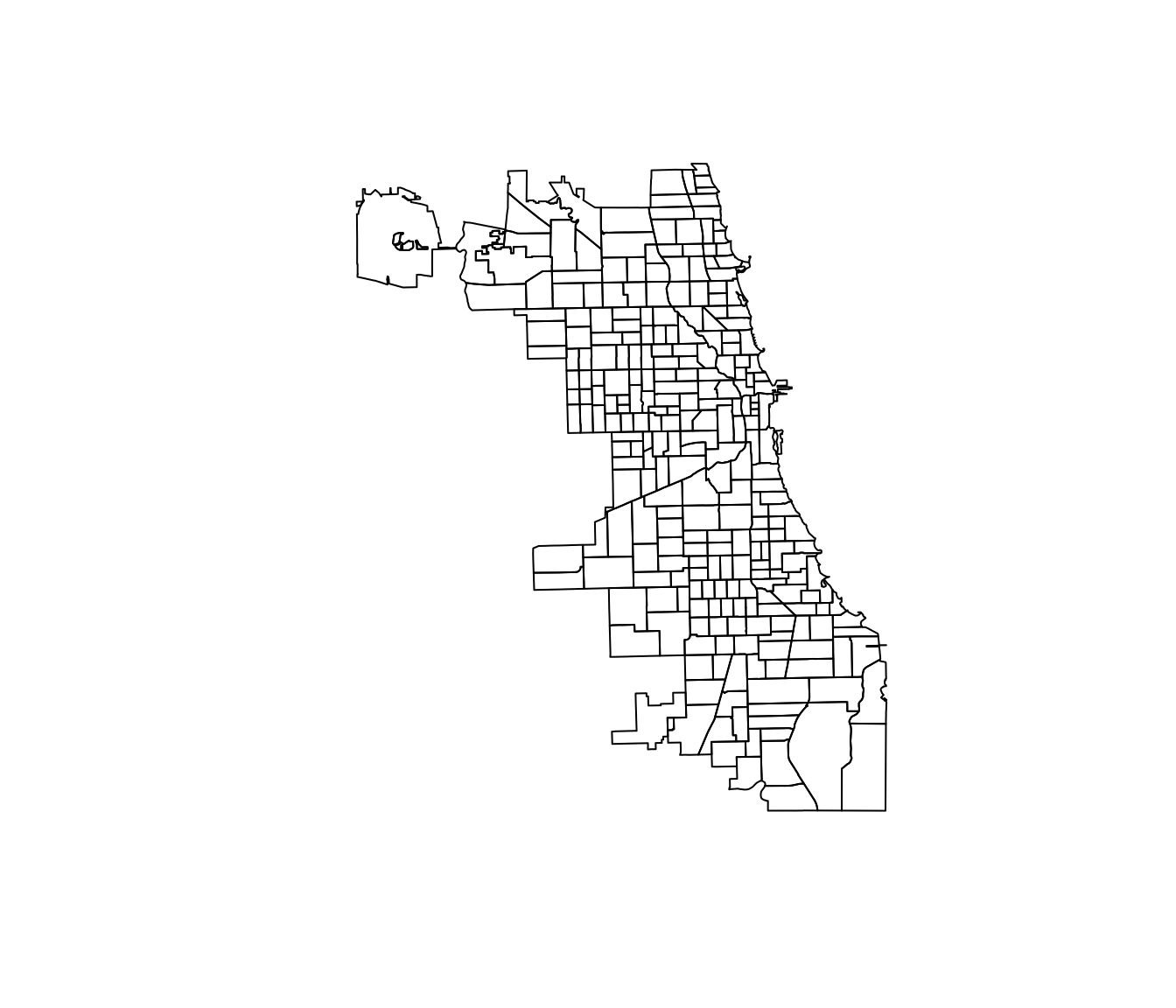
Cool, right? So what does it mean that this “spatial polygons data frame” has dimensions 277 and 4? The first number is generally the number of distinct shapes (features) in the shapefile. In our case, we 277 polygons. And what about the second number? The second number gives us the number of fields—essentially the number of variables (a.k.a. features) for which we have information for each polygon.
Decomposing a shapefile
We can dive a bit deeper into the data that compose a shapefile in R. Up to this point, you’ve seen that you can access the columns of a data.frame4 using the dollar sign, e.g., pretend_df$variable1. Spatial data frames add an additional level—we now have slots. You can still find out the names of the fields (variables) using names(beats_shp), but now you can also find the names of the slots using slotNames(beats_shp):
# Fied/variable names
names(beats_shp)
## [1] "district" "beat_num" "sector" "beat"# Slot names
slotNames(beats_shp)## [1] "data" "polygons" "plotOrder" "bbox" "proj4string"The data slot is a data frame like we’ve seen before, but now there are other slots related to our spatial data: the polygons, the plot order (plotOrder), the bounding box (bbox), and the proj4string (a string that encodes the projection used for the polygons’ coordinates).
Let’s take a look at the data slot. To access the slots, use the slot’s name in conjunction with an ampersat, e.g., beats_shp@data
# Check the class of the object in the 'data' slot
beats_shp@data %>% class()
## [1] "data.frame"# Check the head of the object in the 'data' slot
beats_shp@data %>% head()## district beat_num sector beat
## 0 17 1713 1 1
## 1 31 3100 0 0
## 2 19 1914 1 1
## 3 19 1915 1 1
## 4 19 1913 1 1
## 5 19 1912 1 1# Check the head of the object in the 'data' slot
beats_shp@data %>% dim()## [1] 277 4Let’s see what objects are in the other slots.
# 'plotOrder' slot
beats_shp@plotOrder %>% head()
## [1] 33 253 260 252 2 45# 'bbox' slot
beats_shp@bbox## min max
## x -87.94011 -87.52414
## y 41.64455 42.02303# 'proj4string' slot
beats_shp@proj4string## CRS arguments: +proj=longlat +ellps=WGS84 +no_defsFinally, let’s investigate the polygons slot. What is the class?
# Find the class
beats_shp@polygons %>% class()
## [1] "list"# Find the length of the list
beats_shp@polygons %>% length()## [1] 277A list of length 277! Where have we seen the number 277 before? The dimensions of the beats_shp and the number of rows in the data frame in the data slot. The polygons slot is a list whose elements are the individual polygons that make up the shapefile.
What is the class of a single polygon (a single element of the list in the polygons slot)?5
# Class of the first element in the 'polygons' slot
beats_shp@polygons[[1]] %>% class()
## [1] "Polygons"
## attr(,"package")
## [1] "sp"This polygon object has the class Polygons, which is simultaneously fitting and uninformative. Are you ready to get a bit meta? The polygons in the polygons slot have slots of their own. Let’s see the names of the slots for a single polygon in the polygons slot.
# Slot names for a polygon
beats_shp@polygons[[1]] %>% slotNames()
## [1] "Polygons" "plotOrder" "labpt" "ID" "area"Let’s (quickly) continue down this rabbit hole, accessing the Polygons slot and checking its class.
# What is the class?
beats_shp@polygons[[1]]@Polygons %>% class()
## [1] "list"# What is the length?
beats_shp@polygons[[1]]@Polygons %>% length()## [1] 1Another list, but this list is only of length one. Let’s access the single element in this list and then check the slot names on last time.
# Deep in the rabbit hole
beats_shp@polygons[[1]]@Polygons[[1]] %>% slotNames()
## [1] "labpt" "area" "hole" "ringDir" "coords"Finally, we see a slot name coords. These are the coordinates of the points that make up the first polygon in our shapefile. Let’s check the head and dimensions of this object then plot its points.
# The head of the coordinates
beats_shp@polygons[[1]]@Polygons[[1]]@coords %>% head()
## [,1] [,2]
## [1,] -87.70473 41.97577
## [2,] -87.70472 41.97577
## [3,] -87.70472 41.97574
## [4,] -87.70471 41.97570
## [5,] -87.70470 41.97567
## [6,] -87.70468 41.97565# The dimensions of the coordinates
beats_shp@polygons[[1]]@Polygons[[1]]@coords %>% dim()## [1] 345 2# Plot the coordinates
beats_shp@polygons[[1]]@Polygons[[1]]@coords %>% plot()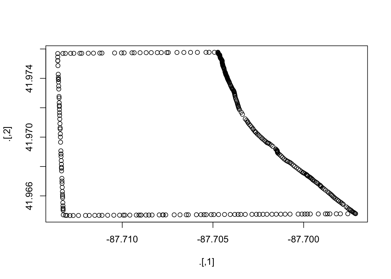
Thus, we see that the first polygon is made up of 345 coordinates that jointly determine area for beat number 1713 (the first row in beats_shp@data). We can confirm that these points match the polygon for beat number 1713 by taking the subset() of beats_shp:
subset(beats_shp, beat_num == "1713") %>% plot()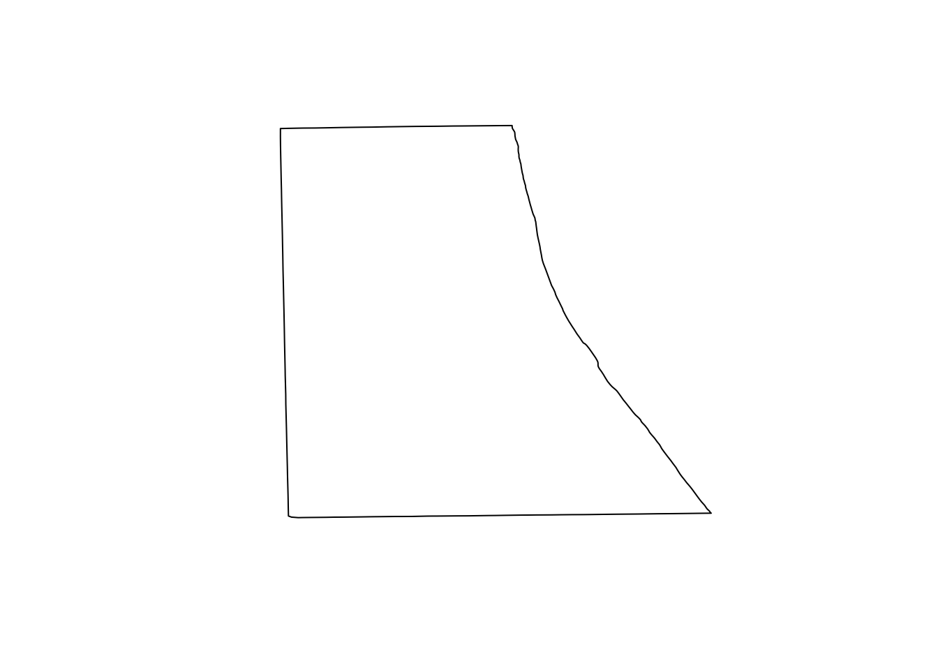
So what have we learned, thus far, about this shapefile? The shapefile is made up of polygons, and each polygon is made up of points on a coordinate system—in this case, longitudes (\(x\)) and latitudes (\(y\)). When you plot the points using their coordinates and then connect the dots (points), you get a polygon. Together, the polygons determine the shapefile. In addition to shapes of the polygons, we also have data (in the data slot) about each polygons. In the current examples, we have four fields/attributes/features/variables6 about the polygons, but in other cases, you will know a lot more about each polygon—for instance, Census will have hundreds of variables for each polygon (the polygons are the Census blocks, tracts, etc.).
Building a shapefile
We can also move in the opposite direction:
- Create a data frame with two columns for the coordinates.
- Convert the data frame to a matrix.
- Convert the matrix of coordinates to a polgyon using
Polygon(). - Create a
Polygonsobject using a list and the functionPolygons(). - Create a
SpatialPolygonsobject from a list thePolygonsobject(s). - Create a
SpatialPolygonsDataFramefrom theSpatialPolygonsobject and a data frame.
# Create coordinates in data.frame
coord_df <- data.frame(
  x = c(0, 0, 1, 2, 1, 1),
  y = c(0, 1, 1, 0, 0, -1))
# Convert data.frame to matrix
coord_mat <- coord_df %>% as.matrix()
# Create a Polygon
the_polygon <- Polygon(coord_mat)
# Create the Polygons object
the_polygons <- Polygons(list(the_polygon), 1)
# Create the SpatialPolygons object
the_sp <- SpatialPolygons(list(the_polygons))
# Create a SpatialPolygonsDataFrame
the_spdf <- SpatialPolygonsDataFrame(the_sp,
  data = data.frame(a = 12, b = 6))
Now let’s check our work:
# Plot 'the_spdf'
plot(the_spdf)
# Check the data slot
the_spdf@data
## a b
## 1 12 6Notes:
- Notice that we created the polygon by plotting the points in the order that they are listed (and connecting the last point to the first point).
- In this example, we created only one polygon, but the process is similar for multiple polygons.
Plotting shapefiles with ggplot2
You’ve already seen that we can use R’s base plot() function to plot shapefiles, but what if we want to use ggplot2? In this situation, ggplot2 still produces pretty pictures, but it can be much slower than plot() when you have a lot of polygons with many points. Plot at your own risk.7
Okay, so let’s plot the police beats shapefile. ggplot2 wants a data frame where each row is a point. As we saw above, we’re almost there—the polygons are composed of points—but we need to formally convert the spatial polygons data frame to a data frame. For this task, I suggest the tidy() function from the broom package.8 We simply feed our shapefile (the spatial polygons data frame beats_shp) to tidy(), and we get back a data frame where each row is a point in one of the polygons in the shapefile. This process can take a while and can also take up a lot of memory if you have many polygons with many points.
# Tidy the shapefile
beats_df <- tidy(beats_shp)
## Regions defined for each Polygons# Look at the first three rows
beats_df %>% head(3)## long lat order hole piece group id
## 1 -87.70473 41.97577 1 FALSE 1 0.1 0
## 2 -87.70472 41.97577 2 FALSE 1 0.1 0
## 3 -87.70472 41.97574 3 FALSE 1 0.1 0Now we are ready to plot. The syntax for ggplot2 remains the same. We need to map the x and y aesthetics (longitude and latitude), as well as the group (the polygon). For the actual plotting, we can use geom_path()—for only the outline of the polygons—and/or geom_polygon(), which allows for filling the polygons with color. geom_map is another nice option, but I will stick to geom_path() and geom_polygon() because they are a bit clearer. Finally, the coord_map() function allows you to specify a projection for the map. If you’ve ever seen maps that look a bit strange, it was probably because they used a different projection.9
# Plot the tidied shapefile
ggplot(data = beats_df, aes(x = long, y = lat, group = group)) +
  geom_polygon(fill = "grey90") +
  geom_path(size = 0.3) +
  xlab("Longitude") +
  ylab("Latitude") +
  ggtitle("Chicago police beats") +
  theme_ed +
  coord_map()
Points data
In addition to shapefiles, the second type of vector data you will often encounter is point data. These files are exactly what they sound like: each observation (row) contains coordinates for a point in space and information on some set of variables.
Let’s load a points dataset. The file chicagoCrime.rds containts Chicago’s police incident reports data from 2010 to the present (again, downloaded from Chicago’s data portal). The actual dataset has a few more variables and goes back to 2001, but I wanted to keep the file a bit smaller. I’ve saved the file as an .rds file, which is an R-specific format that offers a lot of compression, substantially reducing the size of the file. To load an .rds file, you can use the readRDS() function (or readr’s read_rds() function, which is just a wrapper for readRDS()). Let’s load it.
# Read crime points data file
crime_df <- readRDS(paste0(dir_12, "chicagoCrime.rds"))
# Convert to tbl_df
crime_df %<>% tbl_df()
# Check it out
crime_df
## # A tibble: 2,234,883 x 8
## ID Date `Primary Type` Arrest Domestic
## <int> <chr> <chr> <chr> <chr>
## 1 8438081 01/12/2012 06:40:00 PM THEFT true false
## 2 8438082 01/08/2012 12:00:00 PM THEFT false false
## 3 8438084 01/12/2012 07:23:00 PM NARCOTICS true false
## 4 8438085 01/12/2012 04:30:00 PM BATTERY false false
## 5 8438086 01/11/2012 01:00:00 PM CRIMINAL DAMAGE false false
## 6 8438087 01/10/2012 02:00:00 AM ASSAULT false true
## 7 8438088 01/12/2012 05:55:00 PM THEFT true false
## 8 8438089 01/10/2012 04:00:00 PM MOTOR VEHICLE THEFT false false
## 9 8438090 01/12/2012 07:20:00 PM DECEPTIVE PRACTICE true false
## 10 8438091 01/12/2012 07:30:00 PM DECEPTIVE PRACTICE false false
## # ... with 2,234,873 more rows, and 3 more variables: Beat <int>,
## # Latitude <dbl>, Longitude <dbl>Let’s clean up the file a bit more. First, we will change the names of the variables. Second, we will drop any observations missing their latitude or longitude.10 Third, we will convert the dates from character to actual dates using the function mdy_hms() from the lubridate package. The mdy part of the function’s name implies that the dates have month first, followed by day, follwed by year. The hms part of the function’s name implies that we have hours, minutes, and seconds. If you did not have hours, minutes, and seconds, then you would want to use the function mdy(). If you had year, followed by month, followed by day, then you would want to use the function ymd(). And so on….
# Change names
names(crime_df) <- c("id", "date", "primary_offense",
  "arrest", "domestic", "beat", "lat", "lon")
# Drop observations missing lat or lon
crime_df %<>% filter(!is.na(lat) & !is.na(lon))
# Convert dates
crime_df %<>% mutate(date = mdy_hms(date))
## Warning in as.POSIXlt.POSIXct(x, tz): unknown timezone 'zone/tz/2018c.1.0/
## zoneinfo/America/Los_Angeles'# Check it out again
crime_df## # A tibble: 2,203,481 x 8
## id date primary_offense arrest domestic beat
## <int> <dttm> <chr> <chr> <chr> <int>
## 1 8438081 2012-01-12 18:40:00 THEFT true false 131
## 2 8438082 2012-01-08 12:00:00 THEFT false false 1732
## 3 8438084 2012-01-12 19:23:00 NARCOTICS true false 1211
## 4 8438085 2012-01-12 16:30:00 BATTERY false false 1623
## 5 8438086 2012-01-11 13:00:00 CRIMINAL DAMAGE false false 1412
## 6 8438087 2012-01-10 02:00:00 ASSAULT false true 1732
## 7 8438088 2012-01-12 17:55:00 THEFT true false 2513
## 8 8438089 2012-01-10 16:00:00 MOTOR VEHICLE THEFT false false 1723
## 9 8438090 2012-01-12 19:20:00 DECEPTIVE PRACTICE true false 1832
## 10 8438091 2012-01-12 19:30:00 DECEPTIVE PRACTICE false false 1133
## # ... with 2,203,471 more rows, and 2 more variables: lat <dbl>, lon <dbl>Great! While we know that these data depict a points in space, R does not. However, we can easily tell R which variables are the coordinates for these data. For this task, we use the coordinates() function from the sp package (loaded when we load rgdal). You define the coordinates in a data frame using a slightly strange formula of the form coordinates(your_df) <- ~ x_var + y_var. Let’s do it.
# Define longitude and latitude as our coordinates
coordinates(crime_df) <- ~ lon + lat
Check the class, the head, and the slot names of crime_df:
# Check class
crime_df %>% class()
## [1] "SpatialPointsDataFrame"
## attr(,"package")
## [1] "sp"# Check head
crime_df %>% head()## # A tibble: 6 x 6
## id date primary_offense arrest domestic beat
## <int> <dttm> <chr> <chr> <chr> <int>
## 1 8438081 2012-01-12 18:40:00 THEFT true false 131
## 2 8438082 2012-01-08 12:00:00 THEFT false false 1732
## 3 8438084 2012-01-12 19:23:00 NARCOTICS true false 1211
## 4 8438085 2012-01-12 16:30:00 BATTERY false false 1623
## 5 8438086 2012-01-11 13:00:00 CRIMINAL DAMAGE false false 1412
## 6 8438087 2012-01-10 02:00:00 ASSAULT false true 1732# Check slot names
crime_df %>% slotNames()## [1] "data" "coords.nrs" "coords" "bbox" "proj4string"Notice that the variables we defined as the coordinates no longer show up in the head. If you check out the data frame in the data slot, you will not see the variables there, either. (Applying head() to the spatial points data frame is actually giving you the head of the data frame stored in the data slot.) So where did they go? The variables are now stored in the coords slot. See:
# Check out the coords slot
crime_df@coords %>% head()
## lon lat
## 1 -87.63916 41.86449
## 2 -87.71400 41.94883
## 3 -87.68639 41.87963
## 4 -87.76728 41.96173
## 5 -87.71294 41.93927
## 6 -87.72013 41.94916When we converted the data frame to a spatial points data frame—by assigning the coordinates—what happened to the coordinate reference system (CRS)? Did R find/choose a CRS for us?
# Check the projection
crime_df@proj4string
## CRS arguments: NANope. The coordinate reference system is missing. I could not find any information on the CRS that the city of Chicago uses, but let’s assume it matches their other data files—specifically the police beats shapefile we already loaded. We can assign the proj4string using a function by the same name. And we can grab the CRS from another object using the crs() function from the raster package.
# Assing a CRS to the crime points data
proj4string(crime_df) <- crs(beats_shp)
# See if it worked
crime_df@proj4string
## CRS arguments: +proj=longlat +ellps=WGS84 +no_defsGreat!
Points in polygons
Let’s now add the points to our map. Because we have 2.2 million observations, we will focus on two primary offenses: narcotics (200,000+ observations) and homicide (about 3600 observations). dplyr’s handy functions do not currently work on spatial points data frames, but we can use the old-fashioned subset() function, which is like a combination of filter() and select(). Let’s overwrite our current crime_df with the subset that includes only homicides and narcotics.
# Take subset of crimes
crime_df %<>% subset(primary_offense %in% c("HOMICIDE", "NARCOTICS"))
As with the shapefile data, you can quickly plot a spatial points data frame using the base plot() function. Let’s do it.
plot(crime_df)
It looks like we have at least one observation that is not quite in Chicago. From the police beats, we know where Chicago is, so let’s use this knowledge to drop observations that are outside of Chicago.
This observation brings up an important point: with all of the data manipulation required for spatial data—or any data-intensive project—it is good to continually check the quality of your data to make sure everything is making sense. For spatial data, this often looks like making many maps.
First, let’s take the union of all of the polygons, which will give us a single polygon that outlines Chicago. For this task, we will use the function gUnaryUnion() from the rgeos package. We will plot the result using plot().11
# Take the union of the beats polygons
chicago_union <- gUnaryUnion(beats_shp)
# Plot the union
plot(chicago_union)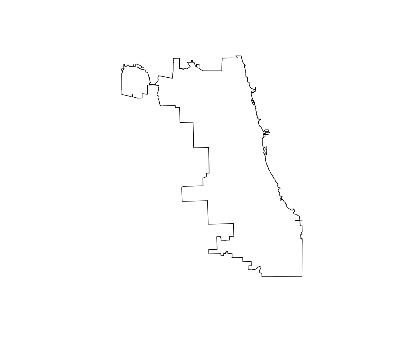
We can now use this union to keep the crimes that fall within Chicago’s city limits.12 In particular, we can use the over() function from the sp package to determine which points are over which polygons.13 Thus, you can also use the over() function to map points to polygons or to grab the value of some variable related to a polygon for each point. Our use is much more simple: if the point is not over a polygon, then we get an NA. This task is sometimes referred to as points in polygons.
# Check which crime points are inside of Chicago
test_points <- over(crime_df, chicago_union)
# From 1 and NA to T and F (F means not in Chicago)
test_points <- !is.na(test_points)
An alternative route that requires a bit more typing:
crime_xy <- crime_df@coords
chicago_xy <- chicago_union@polygons[[1]]@Polygons[[1]]@coords
test_points2 <- point.in.polygon(
  crime_xy[,1], crime_xy[,2],
  chicago_xy[,1], chicago_xy[,2])
Now we will use test_points to drop observations outside of Chicago’s limits.
crime_df <- crime_df[which(test_points == T), ]Finally, let’s plot the crime points again to see if they now fit inside of the city.
plot(chicago_union, col = "grey80")
plot(crime_df, pch = 20, add = T)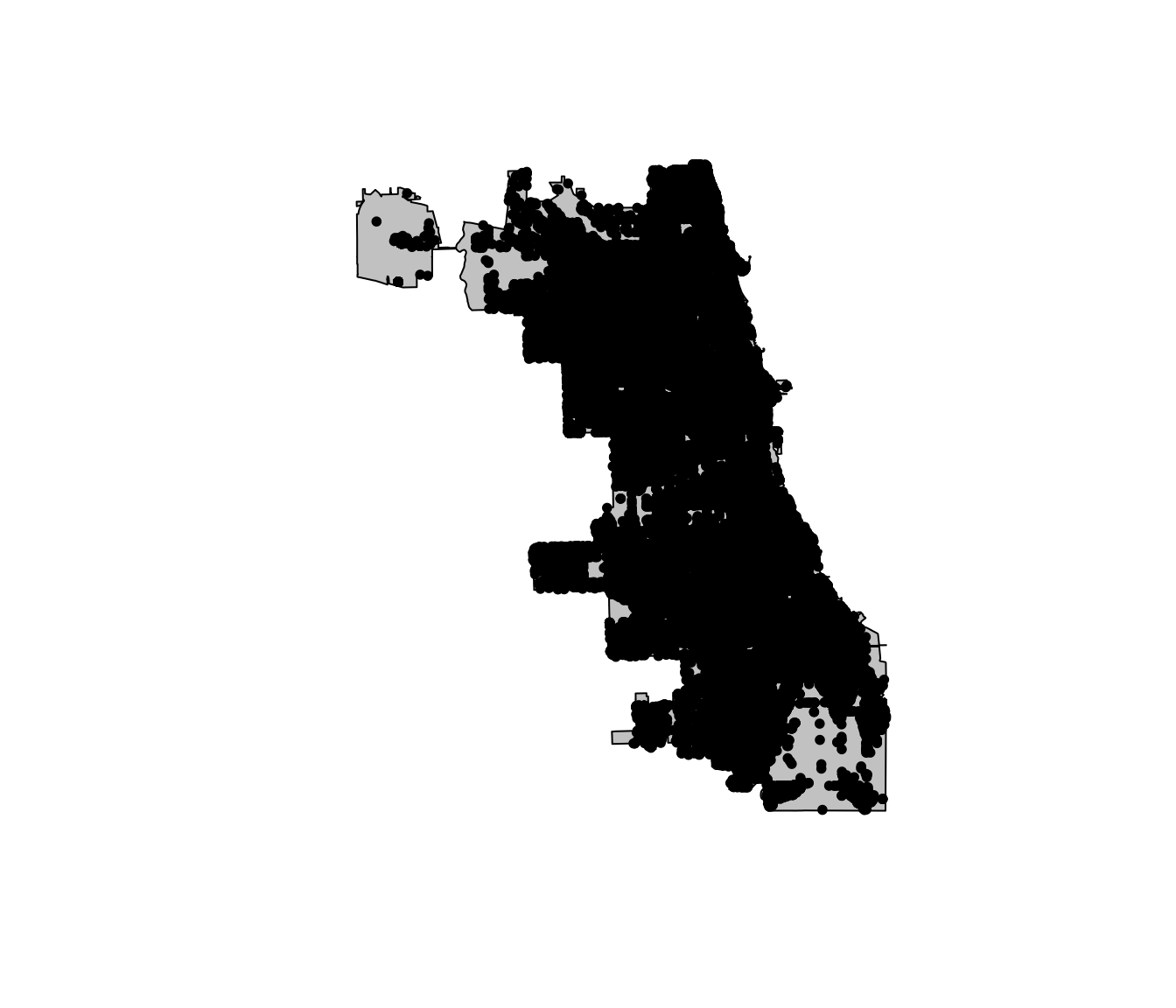
Much better.
But what if we want to do all of this in ggplot2?
Plotting points data with ggplot2
As we discussed above, ggplot2 doesn’t really want spatial data objects—it just wants data frames (or similar objects). Therefore, to plot the spatial points data frame in ggplot2, we want to convert it back to a standard data frame. Because it may be hand to preserve the spatial object, let’s copy the current crime_df, renaming it to crime_spdf and then convert crime_df to a tbl_df.
# Copy the spatial points data frame, renaming
crime_spdf <- crime_df
# Convert the spatial points data frame to tbl_df
crime_df <- crime_df %>% tbl_df()
# Check classes
crime_spdf %>% class()
## [1] "SpatialPointsDataFrame"
## attr(,"package")
## [1] "sp"crime_df %>% class()## [1] "tbl_df" "tbl" "data.frame"Alright, we are now ready to plot the police beat polygons with the crime data. Let’s make a map for each class of crime. I’ll add a factor variable for type of crime. I’ll also add year.
# Add a factor to crime_df
crime_df %<>% mutate(crime_fac =
  factor(primary_offense,
    levels = c("HOMICIDE", "NARCOTICS"),
    labels = c("Homicide", "Narcotics")
    ))
# Add year
crime_df %<>% mutate(year = year(date))
# The maps
ggplot(data = crime_df) +
  geom_path(data = beats_df, aes(long, lat, group = group),
    size = 0.3, color = "grey60") +
  geom_point(aes(lon, lat, color = crime_fac, alpha = crime_fac),
    size = 0.5) +
  xlab("") + ylab("") +
  ggtitle("Spatial distribution of homicides and narcotics offenses",
    subtitle = "Chicago, 2010 to present") +
  theme_ed +
  theme(legend.position = "none", axis.text = element_blank()) +
  scale_color_manual(values = viridis(2, end = 0.6)) +
  scale_alpha_manual(values = c(0.5, 0.05)) +
  coord_map() +
  facet_grid(. ~ crime_fac)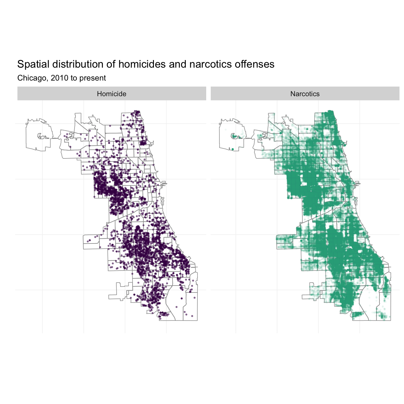
What if we want to incorporate time into this picture? We can add another dimension to the fact_grid(). I’m also going to look only at 2010, 2013, and 2016 to keep things from getting too crazy.
# The maps
ggplot(data = subset(crime_df, year %in% c(2010, 2013, 2016))) +
  geom_path(data = beats_df, aes(long, lat, group = group),
    size = 0.3, color = "grey60") +
  geom_point(aes(lon, lat, color = crime_fac, alpha = crime_fac),
    size = 0.5) +
  xlab("") + ylab("") +
  ggtitle("Spatial distribution of homicides and narcotics offenses",
    subtitle = "Chicago, 2010 to present") +
  theme_ed +
  theme(legend.position = "none", axis.text = element_blank()) +
  scale_color_manual(values = viridis(2, end = 0.6)) +
  scale_alpha_manual(values = c(0.5, 0.1)) +
  coord_map() +
  facet_grid(year ~ crime_fac)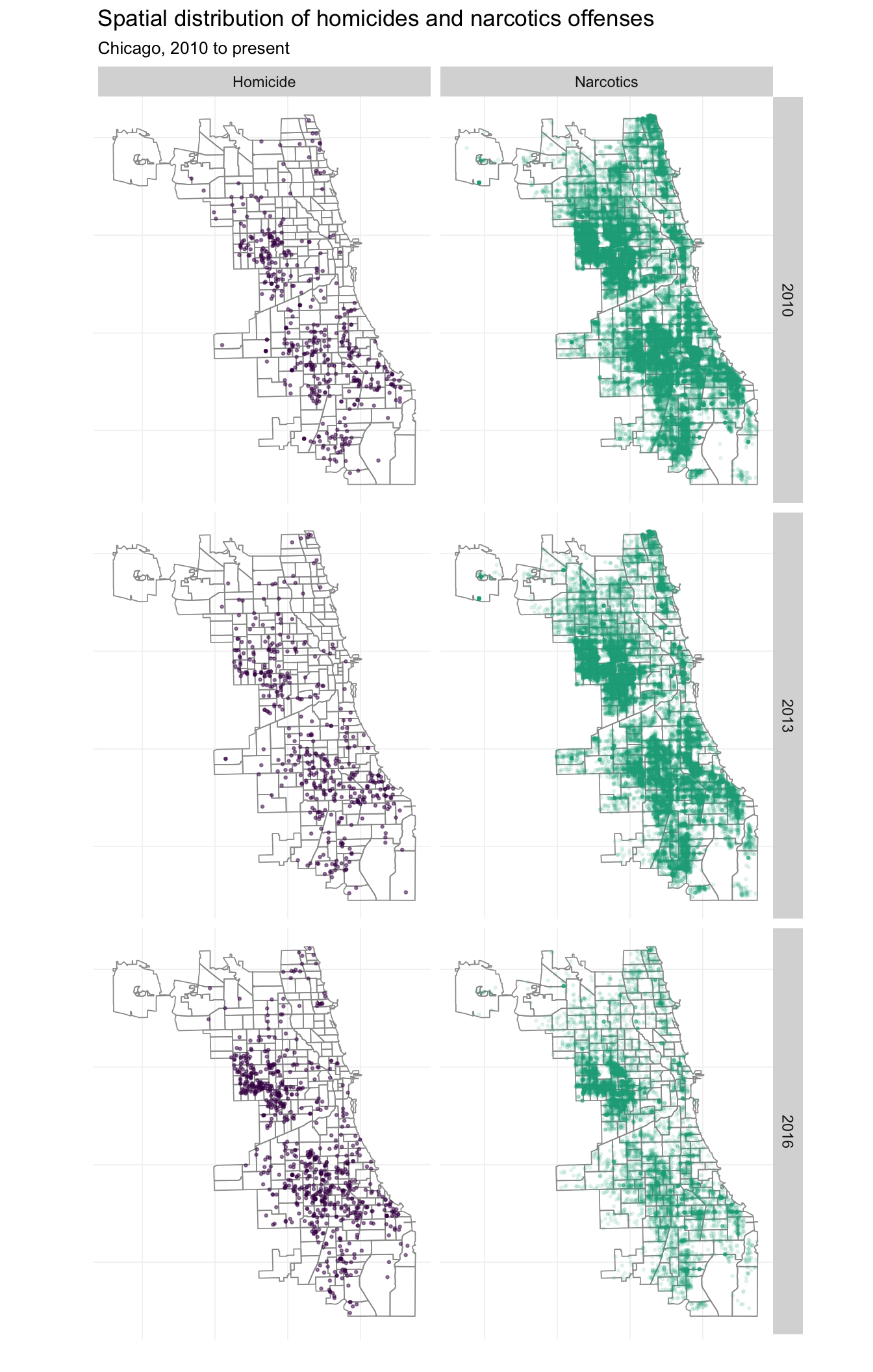
Nice. These maps are pretty interesting—you can see Chicago’s highly publicized homicide explosion in 2016, but you can also see a (non-publicized) large drop in the narcotics busts in 2016.
Aggregating points to polygons
What if want to count the number of incidents within a beat? You could use the over() function from the sp package, but the poly.counts() function in the GISTools package is a bit easier. You feed the function a dataset of points and a dataset of polygons, and poly.counts() counts the points within each polygon.
The general
poly.counts(pts = crime_spdf, polys = beats_shp)Let’s also add a year feature to the spatial points data frame.
# Add 'year' to spatial points data frame
crime_spdf@data %<>% mutate(year = year(date))
Now let’s count the points in each polygon (beat) by year and by type of crime.
# Count homicides by year
homicide_beats <- lapply(X = 2010:2016, FUN = function(y) {
  # Count points in polygons
  tmp <- poly.counts(
    pts = subset(crime_spdf, (year == y) & (primary_offense == "HOMICIDE")),
    polys = beats_shp)
  # Create data frame
  tmp_df <- data.frame(
    id = names(tmp),
    count = tmp)
  # Change names
  names(tmp_df)[2] <- paste0("hom_", y)
  # Return tmp_df
  return(tmp_df)
  })
# Count narcotics offenses by year
narcotics_beats <- lapply(X = 2010:2016, FUN = function(y) {
  # Count points in polygons
  tmp <- poly.counts(
    pts = subset(crime_spdf, (year == y) & (primary_offense == "NARCOTICS")),
    polys = beats_shp)
  # Create data frame
  tmp_df <- data.frame(
    id = names(tmp),
    count = tmp)
  # Change names
  names(tmp_df)[2] <- paste0("narc_", y)
  # Return tmp_df
  return(tmp_df)
  })
Finally, we will (1) bind these lists of datasets together, and (2) join these datasets onto the data stored in the police beats shapefile (in the data slot).
# Bind the lists together
narc_df <- bind_cols(narcotics_beats)
hom_df <- bind_cols(homicide_beats)
# Select unique columns
narc_df <- narc_df[, !duplicated(names(narc_df))] %>% tbl_df()
hom_df <- hom_df[, !duplicated(names(hom_df))] %>% tbl_df()
Finally, we can join these data in hom_df and narc_df to the data slot in our shapefile. We will add the row names to the shapefile’s data so that we can join the dataset with narc_df and hom_df. We will then update beats_df using tidy(). Finally, to join the new variables, we will use left_join() from dplyr. It’s a great function.
# Add row names
beats_shp@data$id <- rownames(beats_shp@data)
# Join the count data
beats_shp@data <- left_join(x = beats_shp@data, y = narc_df, by = "id")
beats_shp@data <- left_join(x = beats_shp@data, y = hom_df, by = "id")
# Re-create data frame
beats_df <- tidy(beats_shp, region = "id")
# Join the beats counts (again)
beats_df %<>% left_join(x = ., y = narc_df, by = "id")
beats_df %<>% left_join(x = ., y = hom_df, by = "id")
And now, we can plot our shapefile, coloring the police beats by the number of homicides in 2016. We will update beats_df.
ggplot(beats_df, aes(long, lat, group = group)) +
  geom_polygon(aes(fill = hom_2016), color = "black", size = 0.07) +
  xlab("") + ylab("") +
  ggtitle("Homicides by police beat, Chicago 2016") +
  theme_ed +
  theme(axis.text = element_blank()) +
  scale_fill_viridis("Homicides within police beat",
    option = "B") +
  coord_map()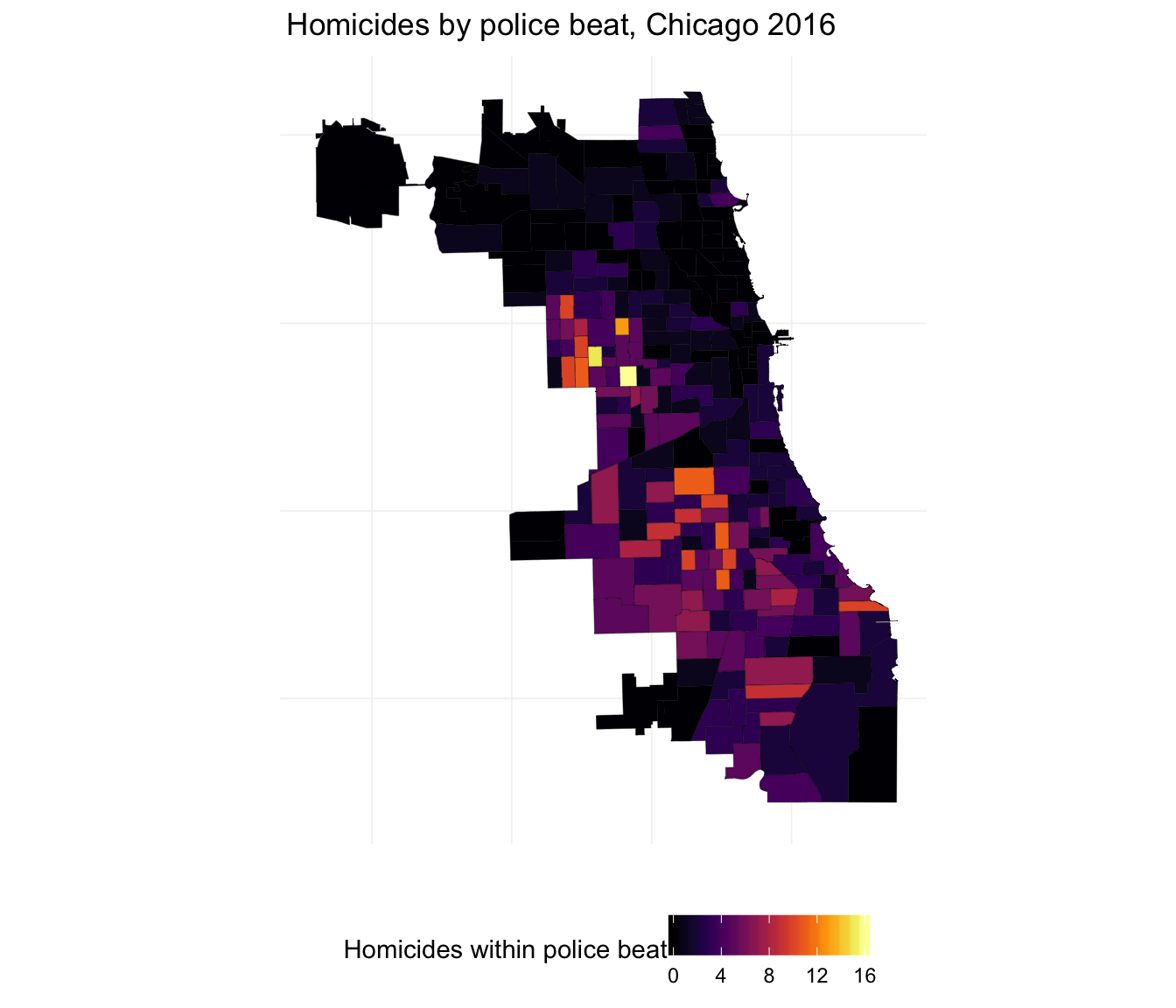
Let’s also plot the within-beat change between 2010 and 2016.
ggplot(beats_df, aes(long, lat, group = group)) +
  geom_polygon(aes(fill = hom_2016 - hom_2010), color = "black", size = 0.07) +
  xlab("") + ylab("") +
  ggtitle("Homicide change between 2010 and 2016, by police beat, Chicago") +
  theme_ed +
  theme(axis.text = element_blank()) +
  scale_fill_viridis("Change in number of homicides within police beat",
    option = "B") +
  coord_map()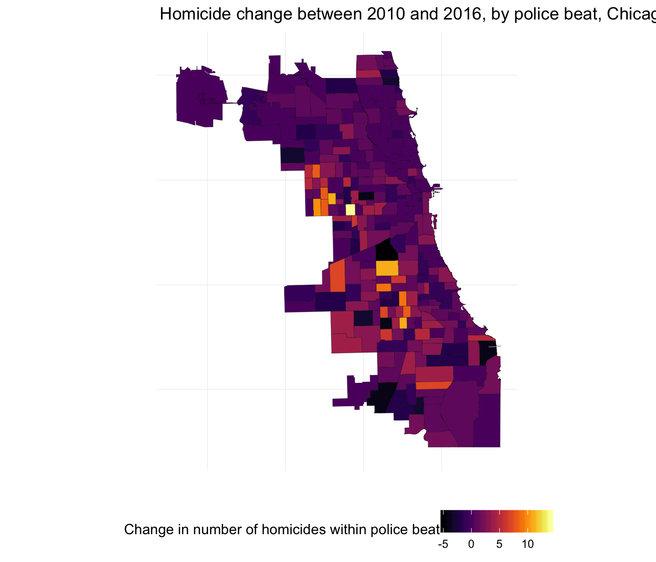
Finally, let’s make the same plots for narcotics.
ggplot(beats_df, aes(long, lat, group = group)) +
  geom_polygon(aes(fill = narc_2016), color = "black", size = 0.07) +
  xlab("") + ylab("") +
  ggtitle("Narcotics by police beat, Chicago 2016") +
  theme_ed +
  theme(axis.text = element_blank()) +
  scale_fill_viridis("Narcotics offenses within police beat",
    option = "B") +
  coord_map()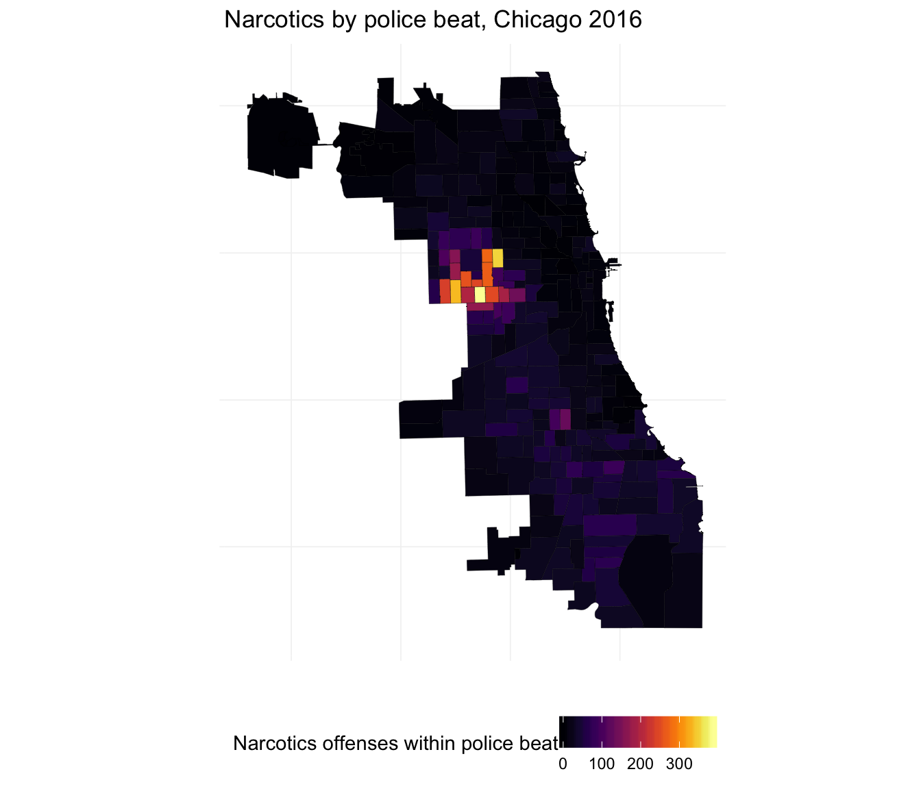
ggplot(beats_df, aes(long, lat, group = group)) +
  geom_polygon(aes(fill = narc_2016 - narc_2010), color = "black", size = 0.07) +
  xlab("") + ylab("") +
  ggtitle("Narcotics change between 2010 and 2016, by police beat, Chicago") +
  theme_ed +
  theme(axis.text = element_blank()) +
  scale_fill_viridis("Change in number of narcotics offenses within police beat",
    option = "B") +
  coord_map()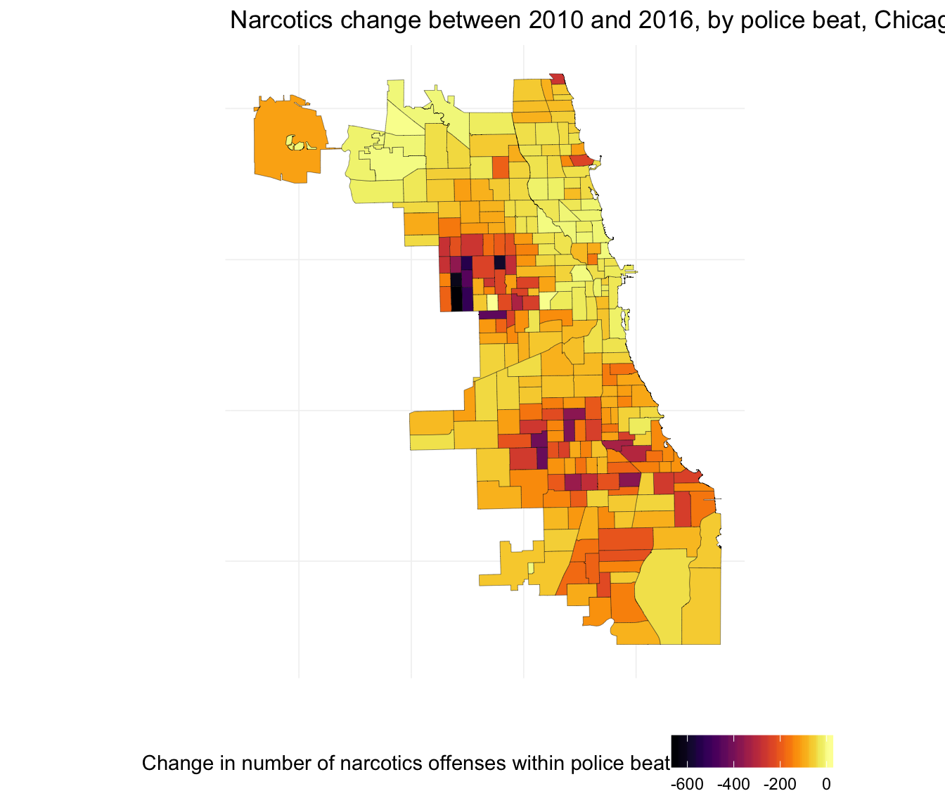
Projections
Let’s return to the proj4string slot for a moment. This slot contains the projection (coordinate reference system or CRS) used in creating the shapefile. Different projections yield different sets of coordinates. Thus, if your projects entails multiple datasets—as most do—then you need to make sure that you are using a consistent projection across all of your datasets/files. If you do not, then (0, 0) in one of your datasets may actually be (180, 180) in another of your datasets—nothing will line up (or it will erroneously line up). Be careful here. For information on how to change projections, see the help files ?raster::crs, ?rgdal::spTransform, the proj4 package, and/or the proj.4 website).
Other resources
If you are interested in learing more about spatial data, check out Sol Hsiang’s course, Public Policy 290.
Here are a few more resources for utilizing spatial data in R.
- http://www.nickeubank.com/wp-content/uploads/2015/10/gis_in_r_vector_cheatsheet.pdf
- https://science.nature.nps.gov/im/datamgmt/statistics/r/advanced/spatial.cfm
- https://www.datacamp.com/courses/working-with-geospatial-data-in-r
- http://www.rspatial.org/
- https://pakillo.github.io/R-GIS-tutorial/
- http://spatial.ly/r/
- https://cran.r-project.org/doc/contrib/intro-spatial-rl.pdf
- ftp://ftp.bgc-jena.mpg.de/pub/outgoing/mforkel/Rcourse/spatialR_2015.pdf
Fun tools: unpaywall
The browser extension unpaywall helps you find papers that are behind a paywall. It doesn’t work all the time, but it works frequently, and I imagine/hope it will continue to get better.
I told you it was important!↩
Fact.↩
I downloaded these data from Chicago’s data portal.↩
or
tibbleortbl_dfordata.table↩Recall that we use
a_list[[n]]to access the nth object of the lista_list.↩I know, too much. I just wanted to emphasize that you will hear different words for the same concept across disciplines.↩
If it is taking too long, try saving the plot, rather than printing it to screen.↩
You can use this
tidy()function for tidying up all kinds of objects.↩See
?coord_mapfor more information.↩In your actual research, you want to be careful with which observations are missing values—it is quite likely that latitude and longitude are not missing at random.↩
The reason we take the union here is that we want a single polygon when testing whether the points are in Chicago. It makes life a bit easier.↩
You could also make use of the bounding box of the shapefile for the exercise, but it would not be as clean—you might still have crimes that are outside of the police beats.↩
Warning: The
over()function can be a bit slow—the task we are asking R to complete can be pretty computationally intense if you have complex shapes for your polygons (many points making up your polygons) and many points to test.↩